Keeping track of follow-up dates manually can get messy fast — especially if you’re juggling multiple contacts. Luckily, with the right formula, you can automate the entire schedule in one go. In this post, you’ll learn how to create an automated follow-up schedule in Google Sheets using a single combination formula. Just enter the first follow-up date, number of follow-ups, and the interval — and let the formula do the rest. No helper columns or manual calculations needed.
What You’ll Need
To create an automated follow-up schedule in Google Sheets, we’ll use a simple table with the following details:
- First follow-up date
- Name of the person
- Contact info (email or phone)
- Number of follow-ups
- How often (in days)
Once you set that up, we’ll use a single formula to generate all future follow-up dates.
Sample Data Setup
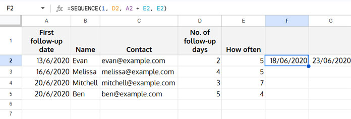
Here’s a quick example of how your input table might look:

This is all we need to build our automated schedule table.
Preview of the Final Follow-Up Table
Let’s take Evan as an example. His first follow-up date is 13/06/2020. You want to follow up with him two more times, every 5 days. So his follow-up dates will be:
- 18/06/2020
- 23/06/2020
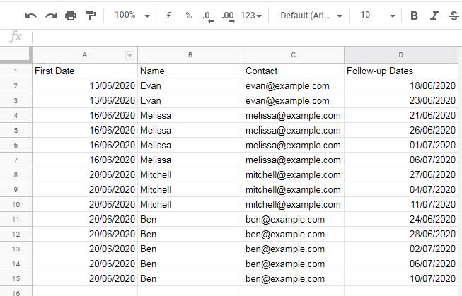
The output table will look something like this:
| First Date | Name | Contact | Follow-up Dates |
|---|---|---|---|
| 13/06/2020 | Evan | [email protected] | 18/06/2020 |
| 13/06/2020 | Evan | [email protected] | 23/06/2020 |
| … | … | … | … |
And all of that is generated automatically with one formula.
The Formula
Assume your input data (like the table above) is in Sheet1, starting from cell A2. In Sheet2, paste the following formula in cell A1:
=LET(
   data, Sheet1!A2:E,
   rept, MAP(CHOOSECOLS(data, 1), CHOOSECOLS(data, 4), CHOOSECOLS(data, 5),
     LAMBDA(x, y, z, SEQUENCE(1, y, x+z, z))),
   pvt, ARRAYFORMULA(SPLIT(FLATTEN(
     CHOOSECOLS(data, 1)&"|"&CHOOSECOLS(data, 2)&"|"&CHOOSECOLS(data, 3)&"|"&rept), "|")),
   VSTACK(HSTACK("First Date", "Name", "Contact", "Follow-up Dates"),
     SORT(FILTER(pvt, CHOOSECOLS(pvt, 4)<>""), 5, 1))
)
Once it generates the schedule, just select the first and last columns, then go to Format > Number > Date to display the dates properly.
How It Works
Even though the formula looks complex, the idea behind it is actually simple. It does two things:
1. It creates the follow-up dates
MAP(...LAMBDA(x, y, z, SEQUENCE(1, y, x+z, z)))x→ the first follow-up date (e.g., 13/06/2020)y→ the number of follow-ups you want (e.g., 2)z→ the interval between follow-ups in days (e.g., 5)
The SEQUENCE function creates a horizontal list of follow-up dates.
For example, if the first date is 13/06/2020, the follow-up count is 2, and the interval is 5, the formula becomes:
=SEQUENCE(1, 2, "2020-06-13" + 5, 5)(based on the syntax: SEQUENCE(rows, columns, start, step))
This generates:
→ 18/06/2020, 23/06/2020
The MAP function applies this logic to each row in your dataset, generating the correct follow-up dates for every contact.
2. It reshapes the data into a vertical table
This part:
SPLIT(FLATTEN(...), "|")It combines all the info from each row (first follow-up date, name, contact, follow-up dates), flattens it into a list, then splits it back into separate columns. So you get one row for each follow-up — nice and clean.
If you’ve seen my post on unpivoting data in Google Sheets, this is the same concept — we’re just applying it to follow-up dates.
3. It filters and sorts the final list
SORT(FILTER(...), 5, 1)This removes empty rows and sorts everything by the follow-up date (ascending), so the schedule is clean and ready to go.
Wrap-Up
That’s it — a fully automated follow-up schedule in Google Sheets, powered by a single combination formula. It’s perfect for staying on top of client communication, task reminders, or any recurring contact schedule.
If you’d like to tweak this further — maybe include dropdowns, add time stamps, or filter by contact — feel free to build on this base. Let the formula do the heavy lifting.


Thank you for this article!
Kind regards.