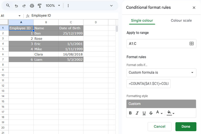
Google Sheets: Highlight If All The Cells Have Content in Range

Published on

To conditionally format a range, I mean to highlight if all the cells have content, you may require a custom formula. The default options in Google Sheets conditional formatting menu may not work for you.

In Google Sheets, advanced level of conditional formatting is possible with custom formulas.

The custom formulas may or may not be complex. But, no doubt, it opens a wide range of custom conditional formatting possibilities.

With custom formulas, you can conditionally highlight a single cell, multiple cells, entire rows, entire columns etc.

Highlight If All The Cells Have Content in Range – What Does It Mean?

See one example of conditional formatting with a custom formula.

My data is in the range A2: E2. What I want to do is highlight all the cells in this range only if all the cells have content.

I mean there should be content in the cells A2, B2, C2, D2, and E2.

The same setting you can apply to multiple rows with a single custom formula.

What is the Use of Such Type of Formatting/Highlighting?

This will help you to easily identify partially filled information in a list/table.

For example, if your data is collected/originated via a Form in Google Sheets, you can highlight the partially filled rows, if any, with my custom formula.

Here is one example of this type of conditional formatting in Google Sheets.

highlight if all the cells have data in Sheets

How to Highlight If All The Cells Have Content in Range

In my example, I have set the range A2: E. If all the five cells in each row are filled, such rows will be highlighted.

The formatting is applied to row-wise like A2: E2, A3: E3, A4: E4 and so on. Not the entire range A2: E but with a single formula.

Can you show me the formula that you have used?

The Custom Google Sheets Formula To Highlight Cells in A Range If All The Cells Have Data In It

Formula:

=counta($A2:$E2)=columns($A$2:$E$2)

To apply this formula, follow the steps detailed below. I know you are already pretty familiar with it.

1. Select the range A2: E.

2. Select Conditional Formatting in Data menu.

3. Apply the above formula in the custom formula field.

format if content in all cells - custom formula setting

4. Click Done.

This way you can make sure that the selected range is highlighted if all the cells in that range have content.

Can you explain to me how this formula conditionally highlight if all the cells have content?

Highlight Row If Filled With Content – Formula Explanation

There are two Google Sheets functions in use. They are COUNTA and COLUMNS and the latter function is optional. I will come to that later.

The COUNTA in Google Sheets counts the content in the selected range. It doesn’t matter the filled data is text, number, date or any other character. It does count.

=counta($A2:$E2)

This formula would return #5 if all the cells have content.

Must Check: Learn All the Count Functions in Google Sheets.

The COLUMNS function can return the number of actual columns in the selected range.

=columns($A$2:$E$2)

This formula would return #5

If all the cells in the range are filled with content, the formula would return TRUE. So the highlighting triggers.

Actually, this formula is enough.

=counta($A2:$E2)=5

I have included the COLUMN function to provide more flexibility. Otherwise, you may need to count the columns in the range manually to input. If you have a large number of columns, this won’t be ideal.

So use the COUNTA and COLUMNS combination formula to conditionally highlight if all the cells have content in range.

Related Reading:

1. Highlight an Entire Row in Conditional Formatting in Google Sheets.

2. Role of Indirect Function in Conditional Formatting in Google Sheets.

3. Conditional Format Based on Group of Data in Google Sheets.

Prashanth KV
Prashanth KV
Your Trusted Google Sheets and Excel Guide Prashanth KV brings a wealth of experience in Google Sheets and Excel, cultivated through years of work with multinational corporations in Mumbai and Dubai. As a recognized Google Product Expert in Docs Editors, Prashanth shares his expertise through insightful blogging since 2012. Explore his blog for practical tips and guidance on maximizing your spreadsheet skills.

Hierarchical Numbering Sequences in Excel

Creating hierarchical numbering sequences in an Excel spreadsheet can significantly improve the way you...

How to Easily Repeat a Sequence of Numbers in Excel

Excel offers multiple ways to accomplish tasks, and the simplicity of each approach depends...

Create a Sequence of Dates at Every Nth Row in Excel (Dynamic Array)

Would you like to create a sequence of dates in every nth row in...

XMATCH Row by Row: Finding Values Across a Range in Google Sheets

Using the BYROW function with XMATCH in Google Sheets allows us to match values...

More like this

XMATCH Row by Row: Finding Values Across a Range in Google Sheets

Using the BYROW function with XMATCH in Google Sheets allows us to match values...

Limit Formula Expansion to a Specific Row in Google Sheets

In this tutorial, I’ll explain how to limit the expansion of an array formula...

3-D Referencing Structured Data Tables in Google Sheets

When you have several tables within a single sheet—not across multiple sheets in a...

LEAVE A REPLY

Please enter your comment!
Please enter your name here

This site uses Akismet to reduce spam. Learn how your comment data is processed.