


")


")

")
")
 in Excel & Google Sheets")


In this tutorial, you’ll learn how to hardcode DateTime criteria in Google Sheets using the FILTER function. If you’re trying to filter data based on exact timestamps (date and time), this guide will show you the right way to format and compare those values.
We’ll walk through practical examples, such as filtering employee attendance logs, to demonstrate how to hardcode DateTime values effectively inside the FILTER function.
Understanding DateTime in Google Sheets
A DateTime value, also called a timestamp, contains both date and time—e.g., 15/01/2022 10:30.
You can format these values in your spreadsheet by selecting the range and going to: Format > Number > Custom date and time
💡 This formatting affects how timestamps are displayed—but it doesn’t change how formulas interpret them internally.
Why FILTER Doesn’t Accept Timestamp Text Strings
In some functions like COUNTIF, you can use a timestamp as a text string:
=COUNTIF(A2:A, ">=16/01/2022 15:30")But FILTER does not reliably interpret text-formatted timestamps. Instead, you should construct DateTime values using the DATE and TIME functions.
Sample Data: Employee Attendance Logs
Let’s say you’re tracking employee attendance with the following timestamped punch-in data:
| Time Logs | Employee Names |
|---|---|
| 15/01/2022 10:30 | Sara |
| 15/01/2022 09:55 | Kristy |
| 15/01/2022 10:00 | Ben |
| 15/01/2022 10:11 | Ronnie |
| 15/01/2022 09:45 | Karen |
| 15/01/2022 09:59 | Tonya |
| 16/01/2022 10:06 | Sara |
| 16/01/2022 09:56 | Kristy |
| 16/01/2022 09:58 | Ben |
| 16/01/2022 10:00 | Ronnie |
| 16/01/2022 10:01 | Karen |
| 16/01/2022 10:05 | Tonya |
Paste this data into cell range A1:B13 in your Google Sheet.
Google Sheets may misinterpret your pasted timestamps depending on your system’s locale or date format. Here’s how to confirm they’re correctly recognized:
To ensure the timestamps are recognized correctly:
- In a blank cell, enter:
=DAY(A2)- If the result is
15, your date format is correct. - If you see an error or an unexpected number, your dates might be stored as text.
- If the result is
- To find the correct format for your spreadsheet:
- Enter
=NOW()in a blank cell. - Note the format of the output (e.g.,
01/15/2022 10:30or15/01/2022 10:30). - Format your time log values in column A to match that style.
- Enter
- Optional: Highlight column A, then go to Format > Number > Date time to apply a standard timestamp format.
This ensures that the FILTER function interprets the values as real DateTime data.
How to Hardcode DateTime Criteria in Google Sheets Filter Function
Example 1: Hardcoding a Full DateTime Condition
To filter rows where timestamps are after 15 January 2022, 3:30 PM, use:
=FILTER(A2:B, A2:A > DATE(2022, 1, 15) + TIME(15, 30, 0))✅ This is the correct way to hardcode a DateTime value inside the FILTER function.
Example 2: Filter Latecomers on a Specific Day
Let’s say office time starts at 10:00 AM. To find employees who punched in after 10:05 AM on 15 January 2022, but before the next day:
=FILTER(A2:B, A2:A > DATE(2022, 1, 15) + TIME(10, 5, 0), A2:A < DATE(2022, 1, 16))Alternative Using ISBETWEEN:
=FILTER(A2:B, ISBETWEEN(A2:A, DATE(2022, 1, 15)+TIME(10, 5, 0), DATE(2022, 1, 16), FALSE, FALSE))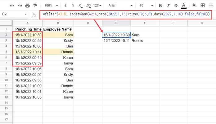
Example 3: Filter Latecomers Regardless of Date
Want to check who arrived after 10:05 AM on any day?
Use this clever trick with MOD to isolate the time part:
=FILTER(A2:B, MOD(A2:A, 1) > TIME(10, 5, 0))Note: MOD(timestamp, 1) removes the date, keeping only the time portion.
Best Practices for Using DateTime in FILTER Function
While this tutorial focuses on hardcoding, a more flexible approach is to place the DateTime value in a cell (e.g., E1) and reference it:
=FILTER(A2:B, A2:A > E1)This makes it easier to update criteria without editing formulas.
Related Resources
If you’re working with timestamps, here are more tutorials related to hardcoding DateTime criteria in Google Sheets and using them in various functions: