By “grouping dates by quarter,” we mean organizing a date column by quarter, then adding additional columns (if any), and aggregating another column.
You can use either a formula-based approach or a pivot table approach to group dates by quarter in Google Sheets. While the formula approach gives you the flexibility to format the data, the pivot table provides a standardized data format.
In the formula-based approach, there are two ways to group by quarter: one using a helper column with various functions and combinations, and another without a helper column (using the QUERY function).
Sample Data
We have the following sample data in A1:C, where A1:C1 contains the headers:
| Date | Item | Amount |
| 20/12/2023 | Apple | 100 |
| 21/12/2023 | Banana | 200 |
| 22/1/2024 | Mango | 150 |
| 22/5/2024 | Orange | 300 |
| 14/6/2024 | Apple | 120 |
| 25/9/2024 | Apple | 180 |
| 26/9/2024 | Apple | 220 |
| 1/10/2024 | Mango | 250 |
| 15/10/2024 | Mango | 130 |
| 09/12/2024 | Mango | 140 |
Group Dates by Quarter Using a Helper Column
1. Extract Quarter and Year
In cell D2, enter the following formula and drag it down to extract the quarter and year from the date:
=IFERROR("Q"&ROUNDUP(MONTH(DATEVALUE(A2))/3,0)&"-"&YEAR(DATEVALUE(A2)))For a detailed explanation of this formula and additional tips, check out Extract Quarter from a Date in Google Sheets: Formulas.
2. Get Unique Quarters
To create a summary report, in cell F2, enter the following formula to get the unique quarters from column D:
=UNIQUE(D2:D)3. Group by Quarter
To group by quarter, use the following SUMIFS formula in cell G2 and drag it down:
=SUMIFS($C$2:$C, $D$2:$D, $F2, $B$2:$B, G$1)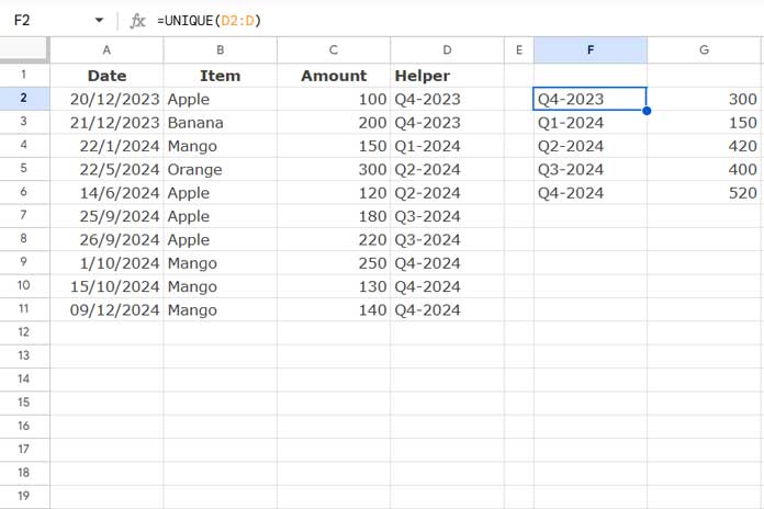
Formula Explanation:
$C$2:$C(sum_range): The range containing the amounts to sum.$D$2:$D(criteria_range1): The range containing the quarters.$F2(criterion1): The specific quarter to match (e.g., “Q1-2024”).
4. Item-Wise Summary
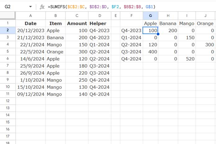
To include item-wise grouping, first, enter this formula in cell G1 to get unique items:
=TRANSPOSE(UNIQUE(B2:B))Then replace the previous formula in cell G2 with this one:
=SUMIFS($C$2:$C, $D$2:$D, $F2, $B$2:$B, G$1)Drag this formula across and down.
Formula Explanation:
$C$2:$C(sum_range): The range containing the amounts to sum.$D$2:$D(criteria_range1): The range containing the quarters.$F2(criterion1): The specific quarter to match (e.g., “Q1-2024”).$B$2:$B(criteria_range2): The range containing the items.G$1(criterion2): The specific item to match (e.g., “Apple”).
Group Dates by Quarter Using QUERY
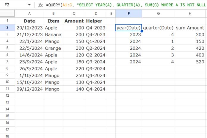
If you prefer not to use a helper column and want to group dates by quarter, QUERY is the best option. Use the following formula:
=QUERY(A1:C, "SELECT YEAR(A), QUARTER(A), SUM(C) WHERE A IS NOT NULL GROUP BY YEAR(A), QUARTER(A)", 1)This QUERY formula groups the dates in column A by Year and Quarter and returns the total of column C (Amount). It filters out blank rows by ensuring A IS NOT NULL.
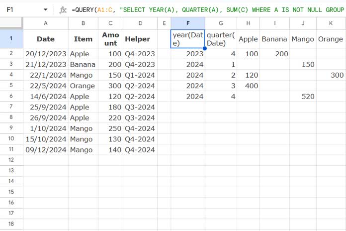
If you want to include the item, use this formula:
=QUERY(A1:C, "SELECT YEAR(A), QUARTER(A), SUM(C) WHERE A IS NOT NULL GROUP BY YEAR(A), QUARTER(A) PIVOT B", 1)The change here is the addition of PIVOT B, which distributes the sum across the unique items in column B (Item), effectively creating a pivot table layout.
It’s that simple!
Note: You might want to modify the header row in the above summary. Learn how to do that by checking out this guide: Understand the Label Clause in Google Sheets Query.
Group Dates by Quarter Using a Pivot Table
This is the simplest approach, as it doesn’t involve any formulas. You can use the built-in pivot table feature to group dates by quarter in Google Sheets.
Steps:
- Select the data range A1:C.
- Click Insert > Pivot Table.
- In the popup, click Create to insert the pivot table into a new sheet.
- Drag and drop Date under Rows.
- If you want to include Items in the grouping, drag and drop Item under Columns (this step is optional).
- Drag and drop Amount under Values.
- Drag and drop Date under Filters.
- Click the dropdown and select Cell is not empty under Filter by Condition.
- Click OK.
- Right-click on any date in the pivot table you just created and select Create Pivot Date Group.
- Select Year-Quarter to group the dates by quarter.
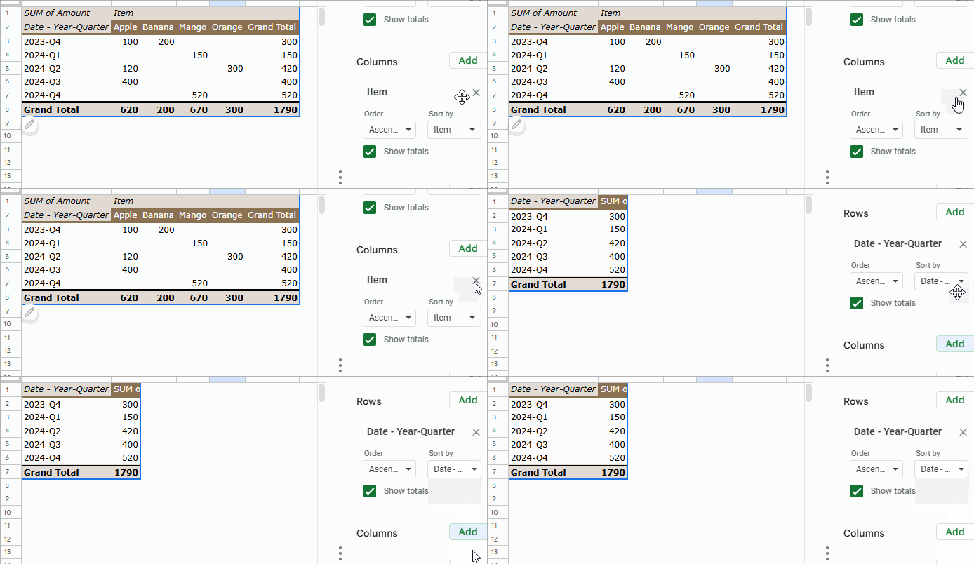
That’s all you need to do!
Resources
- Group Dates in Pivot Table in Google Sheets (Month, Quarter, and Year)
- Query to Create Daily/Weekly/Monthly/Quarterly/Yearly Report Summary in Google Sheets
- Query Quarter Function in Non-Calendar Fiscal Year Data (Google Sheets)
- Convert Dates to Fiscal Quarters in Google Sheets
- Current Quarter and Previous Quarter Calculation in Google Sheets
- How to Calculate Average by Quarter in Google Sheets
- Sum by Quarter in Excel: New and Efficient Techniques


