The MONTH scalar function in Google Sheets QUERY returns month numbers, not month names.
So how do we convert those month numbers into readable month names (text) when summarizing data using QUERY?
If you only want to convert month numbers in a column to month names, see:
Convert Month Numbers to Month Names in Google Sheets
In this tutorial, we focus specifically on returning month names from dates inside QUERY, especially when using GROUP BY, instead of grouping by numeric month values.
This article is a child post of the hub Date Logic in QUERY Function in Google Sheets, which explains date criteria, month-based filtering, and DateTime handling in QUERY.
Sample Data
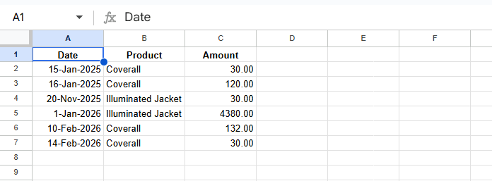
Assume the following source data:

Convert Month Numbers to Month Names in QUERY
There are two valid approaches, depending on how you want the months to be summarized:
- Year-wise Month-wise Summary
(January of each year is summarized separately) - Overall Month-wise Summary
(January of all years is combined)
Year-wise Month-wise Summary (Recommended)
Use this approach when each month should be summarized separately for each year
(e.g., Jan-2025 and Jan-2026 should not be combined).
Step 1: Create a Helper Column (Month Start Date)
Note: You don’t need to test each step separately.
The steps below are shown only to explain how the final QUERY formula is built and why it works.
You can directly use the final formula if you prefer.
=ARRAYFORMULA(IFERROR(EOMONTH(A1:A,-1)+1))This formula returns the first day of the month for each date in column A.
Because it’s wrapped in IFERROR, the result appears as date serial values, not formatted dates — which is perfectly fine for QUERY.
Step 2: Stack the Helper Column with Source Data
=ARRAYFORMULA(HSTACK(A1:C, IFERROR(EOMONTH(A1:A,-1)+1)))Column mapping now becomes:
- Col1 → Date
- Col2 → Product
- Col3 → Amount
- Col4 → Month start date (helper column)
Step 3: Group by Month and Convert to Month Name
=ARRAYFORMULA(
 QUERY(
  HSTACK(A1:C, IFERROR(EOMONTH(A1:A,-1)+1)),
  "select Col4, sum(Col3)
   where Col1 is not null
   group by Col4
   label Col4 'Month', sum(Col3) 'Amount'
   format Col4 'mmm-yyyy'",
  1
 )
)
Result:
| Month | Amount |
| Jan-2025 | 150 |
| Nov-2025 | 30 |
| Jan-2026 | 4380 |
| Feb-2026 | 162 |
Why This Works
- QUERY groups by actual date values (month start dates), not by text.
- The
FORMATclause only affects display, not grouping. - The underlying values remain dates, ensuring correct sorting and chronology.
You can change the display format:
'mmm-yyyy'→ Jan-2017'mmmm yyyy'→ January 2017'mm'→ Numeric month
Overall Month-wise Summary (Across Years)
Use this approach when the same month from different years should be combined
(e.g., January 2025 + January 2026 → one total).
Step 1: Create Two Virtual Columns
=ARRAYFORMULA(IFERROR(TEXT(DATEVALUE(A1:A), "MMMM")))   // Month name (text)
=ARRAYFORMULA(IFERROR(MONTH(DATEVALUE(A1:A))))         // Month number
Why DATEVALUE() is important
Without DATEVALUE(), empty cells are coerced to 0, which Google Sheets interprets as December (month 12).
Using DATEVALUE() with IFERROR() ensures that empty rows remain empty and are not misclassified as December.
Step 2: Stack Data with Virtual Columns
=ARRAYFORMULA(
 HSTACK(
  A1:C,
  IFERROR(TEXT(DATEVALUE(A1:A), "MMMM")),
  IFERROR(MONTH(DATEVALUE(A1:A)))
 )
)
Column mapping:
- Col4 → Month name (text)
- Col5 → Month number (1–12)
Step 3: QUERY with Grouping and Ordering
=ARRAYFORMULA(
 QUERY(
  HSTACK(A1:C, IFERROR(TEXT(DATEVALUE(A1:A), "MMMM")), IFERROR(MONTH(DATEVALUE(A1:A)))),
  "select Col4, Col5, sum(Col3)
   where Col1 is not null
   group by Col4, Col5
   order by Col5
   label Col4 'Month', sum(Col3) 'Amount'",
  1
 )
)
Result:
| Month | Amount | |
| January | 1 | 4530 |
| February | 2 | 162 |
| November | 11 | 30 |
Step 4: Remove the Helper Month-Number Column
=ARRAYFORMULA(
 CHOOSECOLS(
  QUERY(
   HSTACK(A1:C, IFERROR(TEXT(DATEVALUE(A1:A), "MMMM")), IFERROR(MONTH(DATEVALUE(A1:A)))),
   "select Col4, Col5, sum(Col3)
    where Col1 is not null
    group by Col4, Col5
    order by Col5
    label Col4 'Month', sum(Col3) 'Amount'",
   1
  ),
  1, 3
 )
)
This produces a clean output with:
- Month name
- Total amount (combined across years)
Key Takeaways
- The QUERY
MONTH()function returns zero-based month numbers. - Formatting changes appearance, not grouping logic.
- For year-wise summaries, group by month start dates.
- For overall summaries, use a helper month number for sorting.
DATEVALUE()prevents empty cells from being misinterpreted as December.
Final Notes
Use the year-wise method when month values must remain distinct across years, and the overall method when you want to aggregate the same month across all years.
The year-wise method groups by date values, while the overall method groups by month text with a helper month number used for correct ordering. Formatting only affects display, not calculation.


