")
")


")


")

")
")
 in Excel & Google Sheets")


To find the nth largest value from a range or array, use the LARGE function in Google Sheets. For example, the following formula returns 11 as the largest value in the array:
=LARGE({5, 4, 10, 6, 11}, 1)You can also return multiple large values in a single formula by using the LARGE function in combination with the ARRAYFORMULA function.
For example, the following formula returns the largest 3 values:
=ArrayFormula(LARGE({5, 4, 10, 6, 11}, {1; 2; 3}))Syntax:
LARGE(data, n)Arguments:
data– The array or range containing the data set to evaluate.n– The rank from largest to smallest.
Examples of Using the LARGE Function in Sheets
Assume you have student names in one column and their marks in another. You can use the LARGE function to find the top scorers.
In the following example, the names are in A2:A11, and the marks are in B2:B11.
We’ve used the following formulas to find the 1st, 2nd, and 3rd top scorers:
=LARGE(B2:B11, 1) // returns 100
=LARGE(B2:B11, 2) // returns 99
=LARGE(B2:B11, 3) // returns 98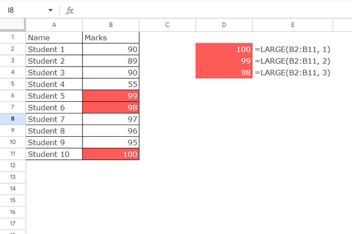
If you want to return the top three scorers using a single formula, you can use this one:
=ArrayFormula(LARGE(B2:B11, {1; 2; 3}))Using the LARGE Function with the FILTER Function
A common use case for the LARGE function is combining it with the FILTER function.
When combining the FILTER and LARGE functions, you can filter a range for rows where the values fall above or equal to the nth largest value in a column of that range.
For example, using the student names and marks mentioned earlier, you can retrieve the top 3 students and their marks with the following formula:
=FILTER(A2:B11, B2:B11>=LARGE(B2:B11, 3))Here, the FILTER function filters the range A2:B11 based on the condition B2:B11 >= LARGE(B2:B11, 3). This condition returns TRUE for rows where the marks in B2:B11 are greater than or equal to the third-largest value.
Another example:
=FILTER(A2:D5, C2:C5=LARGE(C2:C5, 1))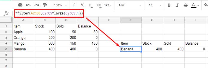
This formula filters the range A2:D5, where the values in C2:C5 are equal to the largest value in that range.
LARGE with XLOOKUP
You can use the LARGE function in combination with the XLOOKUP function to find the nth largest value in a column and return the corresponding value from another column.
For example, the following formula will search for the top scorer in column B and return the student’s name from column A:
=XLOOKUP(LARGE(B2:B11, 1), B2:B11, A2:A11)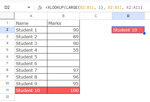
Where:
LARGE(B2:B11, 1)is the search key (the largest value).B2:B11is the lookup range (marks).A2:A11is the result range (student names).
What Happens When the Range is Empty?
When the data range is empty, the LARGE function will return a #NUM! error. You’ll encounter the same issue if the specified nth value (n) is unavailable in the range.
To handle this, you can use the IFERROR function to return either an empty cell or a custom message.
=IFERROR(LARGE(B2:B11, 11))— returns an empty cell.=IFERROR(LARGE(B2:B11, 11), "Your Text Here")— returns a custom message.