To retrieve the latest non-blank value by date, there is no built-in function in Google Sheets. You can code one formula using the native functions in it.

When there are multiple data records (rows) pertaining to a category (user or item), you may need to find the latest non-blank value among them by date.

For example, assume you purchased 1 liter each of cooking oil on 25/07/2023, 06/08/2023, and 23/08/2023, and the prices are $3.52, $4.00, and empty.

The price of the last purchase is left empty because you lost the bill. Then, the most recent purchase price returned by the formula should not be empty, but $4.00.

We usually encounter this issue when we use Google Forms to collect data in Google Sheets. For example, a user might submit the form twice to update the data they submitted earlier.

Such tables will typically contain a date or timestamp column and a category column. We may need to look up a category by the most recent date and return values from other columns in the table.

The advanced lookup functions in Google Sheets, such as XLOOKUP and XMATCH, cannot be used for this.

The best way to solve this problem is to use a combination of the FILTER and SORT functions or an advanced array formula.

Must Check: Google Sheets Function Guide.

The FILTER and SORT combination can find data related to one category (item). If there are multiple users or items, you may need to use my advanced array formula to extract the latest non-blank values by date.

Non-Array Formula to Get the Latest Non-Blank Value by Date in Google Sheets

We will see two examples. In the first example, we have three columns: a date or timestamp column, a category column, and a third column with the values that we want to return.

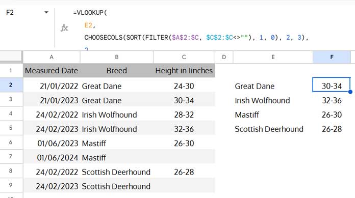
The field labels in cells A1, B1, and C1 are “Measured Date”, “Breed”, and “Height in Inches”, respectively. There is relevant data in the cells below.

To find the latest height of dog breeds from the non-blank cells, we can use the following non-array formula in cell F2:

=INDEX(SORT(FILTER(HSTACK($A$2:$A,C$2:C),($B$2:$B=$E2)*(C$2:C>0)),1,0),1,2)

Where:

• A2:A is the range of cells containing the measured dates.
• B2:B is the range of cells containing the breed names.
• C2:C is the range of cells containing the height in inches.
• E2 is the cell that contains the criterion (breed name).

I’ve copied and pasted the formula down to return the height of other dog breeds from the non-blank cells.

What if there is another column, for example, D2:D, that contains the weight of dog breeds in pounds?

The above Google Sheets formula can return the latest non-blank value by date from multiple columns. You just need to copy and paste the formula down and across.

How does the formula return the latest non-blank value by date in Google Sheets?

Formula Explanation

The HSTACK function is used to combine the first and last columns from the three-column table, which are the Measured Date and Height in Inches.

HSTACK Syntax: HSTACK(range1, [range2, …])

HSTACK($A$2:$A,C$2:C)

This range is used as the input to the FILTER function, which filters out rows that do not meet the specified criteria.

FILTER Syntax: FILTER(range, condition1, [condition2, …])

The criteria (condition1) in this case, the breed name in cell E2 must match the breed name in the second column of the range. Additionally (condition2), the Height in Inches must be greater than 0.

FILTER(HSTACK($A$2:$A,C$2:C),($B$2:$B=$E2)*(C$2:C>0))

The SORT function then sorts the filtered range of cells by the measured dates in descending order.

SORT Syntax: SORT(range, sort_column, is_ascending, [sort_column2, …], [is_ascending2, …])

SORT(FILTER(HSTACK($A$2:$A,C$2:C),($B$2:$B=$E2)*(C$2:C>0)),1,0)

Finally, the INDEX function returns the value from the first row of the sorted range, which is the latest value by date.

INDEX Syntax: INDEX(reference, [row], [column])

Array Formula to Get the Latest Non-Blank Value by Date in Google Sheets

If you use an array formula, you don’t need to specify the breed names (criteria) in cell E2:E.

The formula will take care of everything. It will return two columns, including the breed names.

Here is the array formula that you should enter in cell E2 to get the latest non-blank height of dog breeds:

=LET(range,A2:C,distinct,UNIQUE(CHOOSECOLS(range,2)),IFERROR(HSTACK(distinct,MAP(distinct,LAMBDA(r, BYCOL(CHOOSECOLS(SORT(FILTER(HSTACK(CHOOSECOLS(range,1),CHOOSECOLS(range,{3})),CHOOSECOLS(range,2)=r),1,0),{2}),LAMBDA(c,CHOOSEROWS(TOCOL(c,1),1))))))))

Where:

• A2:C is the data range, where A2:A contains the dates (measured dates), B2:B contains the categories (dog breed names), and C2:C contains the return value (height in inches).

Similar to the non-array formula, this array formula is also capable of returning the latest non-blank value by date from multiple columns in Google Sheets.

To return the height in inches and weight in pounds, similar to the example in Figure 2 above, you need to make the following changes to the formula:

1. Replace the range A2:C with A2:D.
2. Change CHOOSECOLS(range, {3}) to CHOOSECOLS(range, {3, 4}). This means that the third and fourth columns in the range A2:D are the result columns.
3. Change the array {2} to {2, 3}. This means that the second and third columns in the range {A2:A, C2:D} are the result columns.

If you want to return values from 3 columns, the range will become A2:E, CHOOSECOLS(range, {3}) will become CHOOSECOLS(range, {3, 4, 5}) and {2} will become {2, 3, 4}.

Formula Logic

For explanation purposes, we will split the formula into two parts. One part will go into cell E2 and the other part will go into cell F2.

The following UNIQUE formula in cell E2 returns the unique breeds in cell E2:E.

=UNIQUE(B2:B)

The following non-array formula in cell F2 will return the latest non-blank value, i.e., height, by the date of the breed in cell E2.

=CHOOSEROWS(TOCOL(CHOOSECOLS(SORT(FILTER(HSTACK($A$2:$A,$C$2:$C),$B$2:$B=$E2),1,0),2),1),1)

By using the BYCOL function in the above formula, we can make it return the latest non-blank value in the additional column, weight. In other words, we can expand the formula to the right.

Here is the modified formula in cell F2:

=BYCOL(C2:D,LAMBDA(c,CHOOSEROWS(TOCOL(CHOOSECOLS(SORT(FILTER(HSTACK($A$2:$A,c),$B$2:$B=$E2),1,0),2),1),1)))

We need to expand the formula to all rows (E2:E). For that, we can use the MAP function.

=MAP(E2:E,LAMBDA(r, BYCOL(C2:D,LAMBDA(c,CHOOSEROWS(TOCOL(CHOOSECOLS(SORT(FILTER(HSTACK($A$2:$A,c),$B$2:$B=r),1,0),2),1),1)))))

The master array formula is a combination of the above E2 and F2 formulas. The master formula seems different because of the use of LET to name ranges and expressions.

That’s all about retrieving the latest non-blank value by date. Here is the sample sheet for your reference.

Sample_Sheet_28823