Get the First Numeric Value in a Range in Google Sheets

When working with data in Google Sheets, you may need to get the first numeric value in a range to simplify your calculations. This is especially useful when dealing with mixed data types, blank cells, or text entries in a range.

Google Sheets offers several ways to extract the first numeric value in a range, and in this post, we’ll discuss three approaches, starting with the most efficient option.

Generic Formula

The formula to extract the first numeric value in a range is:

=+FILTER(range, ISNUMBER(range))

In this formula, you can replace range with either a row or column (one-dimensional). The formula will return the first numeric value it encounters.

You can also use SINGLE(), an undocumented function, to achieve the same result. The formula becomes:

=SINGLE(FILTER(range, ISNUMBER(range)))

Both formulas will return the first numeric value in a range, with the SINGLE() function or the + operator ensuring that only the first value is returned.

Example: Get the First Numeric Value in a Range in Google Sheets

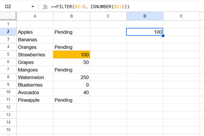
Consider the following example where column B2:B contains mixed data types, including numbers, text, and empty cells. The first numeric value is 100.

To extract that value, you can use the formula:

=+FILTER(B2:B, ISNUMBER(B2:B))

Example of Extracting the First Numeric Value in a Range in Google Sheets

Here’s how the formula works:

The ISNUMBER function returns an array of TRUE or FALSE values, with TRUE representing numeric values.
The FILTER function filters the values in B2:B based on the condition provided by ISNUMBER. This results in only the numeric values being extracted.
The + sign ensures that only the first value returned by the FILTER function is selected.

Alternatively, using SINGLE():

=SINGLE(FILTER(B2:B, ISNUMBER(B2:B)))

Both formulas work for single rows or columns. Simply adjust the range as needed.

Additional Options for Extracting the First Numeric Value

If you’re troubleshooting formulas or seeking alternative solutions, here are two other methods to extract the first numeric value in a range:

1. Using XLOOKUP:

=ARRAYFORMULA(XLOOKUP(TRUE, ISNUMBER(B2:B), B2:B))

The role of the ISNUMBER function is the same as earlier: to return TRUE for numbers and FALSE for other values.

XLOOKUP searches for the key TRUE in the range returned by ISNUMBER, which contains TRUE/FALSE values. It then returns the first corresponding value from the range B2:B.

ARRAYFORMULA is used because ISNUMBER requires array support for operations like XLOOKUP. However, when used within functions like FILTER, INDEX, or SORT, this support is not necessary.

2. Using INDEX-XMATCH:

=INDEX(B2:B, XMATCH(TRUE, ISNUMBER(B2:B)))

XMATCH finds the position of the first TRUE value in the array returned by ISNUMBER.
INDEX then extracts the value at that position in the range B2:B.

Both these formulas work for single rows or columns—just adjust the range as needed.

Conclusion

In this post, we’ve covered several methods to get the first numeric value in a range in Google Sheets, including a generic formula, as well as alternative options like XLOOKUP and INXEX-XMATCH. Whether you’re working with rows or columns, these formulas can help you extract the first numeric value efficiently.

Get the First Text Value in a Range in Google Sheets