")
")


")


")

")
")
 in Excel & Google Sheets")


The GESTEP function in Google Sheets is categorized as an Engineering function. It returns 1 or 0, depending on whether a value (number or date) is greater than or equal to a step (threshold) value.
For example, suppose column A in your sheet contains a list of numbers. You want to check whether those numbers are greater than or equal to a threshold value (or multiple threshold values). In such cases, this Engineering function will be useful.
Another example is when you have target dates for tasks and actual completion dates. Here, you can use the GESTEP function to test whether the completion dates meet or exceed the target dates.
However, you don’t always need to use the GESTEP function to solve the above scenarios in Google Sheets.
Sometimes, using an IF logical function or a simple comparison operator like >= (greater than or equal to) can achieve the same results.
After covering the syntax and arguments, you’ll find several GESTEP formula examples, including how to use the function with or without the ARRAYFORMULA function.
GESTEP Function in Google Sheets – Syntax and Arguments
Syntax:
GESTEP(value, [step])Arguments:
- value: The value (number or date) to test against the step (threshold) value.
- step: The step (threshold) value. It defaults to 0. This means if you skip this argument, the function will consider the step value as 0.
Note:
The function returns 1 (one) if value is greater than or equal to step; otherwise, it returns 0 (zero).
I’ve already explained the purpose of the GESTEP function in Google Sheets above. Now, let me illustrate its use with some example formulas.
GESTEP Formula Examples
Refer to the table below for some basic examples. The ‘values’ are in column A, and the ‘step’ values are in column B.
The results are shown in column C, while the formulas used to calculate them are displayed in column D.
| A | B | C | D | |
| 1 | value | step | result | formula |
| 2 | 5 | 4 | 1 | =GESTEP(A2, B2) |
| 3 | 10 | 10 | 1 | =GESTEP(A3, B3) |
| 4 | 5 | 6 | 0 | =GESTEP(A4, B4) |
| 5 | 10 | 1 | =GESTEP(A5) =GESTEP(A5, B5) | |
| 6 | -10 | -15 | 1 | =GESTEP(A6, B6) |
| 7 | 25/05/2020 | 20/05/2020 | 1 | =GESTEP(A7, B7) |
If there are multiple ‘values’ and corresponding ‘step’ values as shown in the above table, you can simplify the calculations using an ARRAYFORMULA in cell C2:
=ARRAYFORMULA(GESTEP(A2:A7, B2:B7))Ensure that the range C3:C7 is empty to allow the array formula to expand and display the results.
This array formula introduces new possibilities for using the GESTEP function in Google Sheets. How?
With an array formula, you can check whether numbers or dates in a list are greater than or equal to a single step value (threshold value). Here’s how:
Using the array formula above, suppose the values to check are in the range A2:A6, but the step value is fixed at 5.
The following formula checks whether the values in the given range are greater than or equal to the step value of 5:
=ARRAYFORMULA(GESTEP(A2:A7, 5))Formula Alternatives – IF Logical and Comparison Operators
As far as I know, other than using comparison operators or their equivalent functions, there are no direct formula alternatives to the GESTEP function in Google Sheets.
In the table, you can replace the GESTEP array formula in cell C2 with any of the following formulas:
=ARRAYFORMULA((A2:A7>=B2:B7)*1)=ARRAYFORMULA(GTE(A2:A7, B2:B7)*1)=ARRAYFORMULA(IF(A2:A7>=B2:B7, 1, 0))
Additional Tip: GESTEP Formula within the FILTER Function in Google Sheets
I’m concluding this post with an example using the FILTER function.
I have a few tasks listed in column A, with their target completion dates in column B. In column C, you’ll find the actual completion dates of those tasks (please refer to the screenshot below).
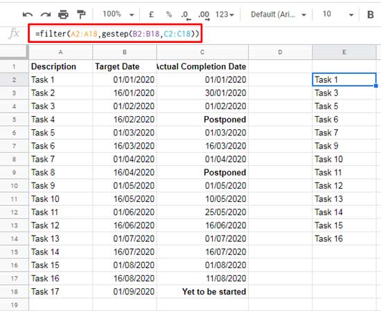
How can you filter only the tasks completed on or before their target dates?
The following formula, combining FILTER and GESTEP, does the job:
=FILTER(A2:A18, GESTEP(B2:B18, C2:C18))Notes:
- The GESTEP function in Google Sheets will return a
#VALUE!error if either thevalueorstepargument is a string. In this example, the FILTER function automatically skips rows in column C that contain strings. - The actual completion date in column C should not be left blank, as blank cells are treated as 0.
For your reference, in cell B2, I’ve used the following formula to generate bimonthly target dates:
=FILTER(
     SEQUENCE(250, 1, DATE(2020, 1, 1), 1),
     (DAY(SEQUENCE(250, 1, DATE(2020, 1, 1), 1)) = 16) +
     (DAY(SEQUENCE(250, 1, DATE(2020, 1, 1), 1)) = 1)
)
That’s all about how to use the GESTEP function in Google Sheets. Enjoy exploring its possibilities!