


")


")

")
")
 in Excel & Google Sheets")


When working with data in Google Sheets, you may encounter duplicate rows. Instead of manually consolidating the data, you can use a formula to automatically combine duplicate rows while retaining all relevant information from other columns
Of course, you can use the UNIQUE function to remove duplicate records if all columns match exactly. You can also use SORTN to remove duplicates based on specific columns. But what if some columns contain different data?
The first approach retains all duplicate rows, while the second approach removes them, potentially leading to data loss. The same happens when using Data menu > Data cleanup > Remove duplicates.
For example, if a customer appears multiple times with different email addresses or phone numbers, you can merge those details into a single row while keeping all relevant information intact.
Sample Table
| Customer ID | Name | Phone | |
| 1 | Samantha | Samantha@temp.com | |
| 1 | Samantha | Samantha_123@temp.com | 123-456-7800 |
| 1 | Samantha | Samantha_123@temp.com | 123-456-7800 |
Here, Customer ID 1 appears three times.
If you apply UNIQUE to this table, it will keep all records:
=UNIQUE(A2:D)If you apply SORTN, it will retain only the first record:
=SORTN(A2:D, 9^9, 2, 1, TRUE)However, neither approach is ideal because they either keep unnecessary duplicates or remove data we want to retain. Instead, we need a method to combine duplicate rows in Google Sheets while keeping all relevant details. The expected output should be:
| Customer ID | Name | Phone | |
| 1 | Samantha | Samantha@temp.com Samantha_123@temp.com | 123-456-7800 |
Sample Data to Combine Duplicate Rows
Here is the sample dataset (A1:D) with the headers Customer ID, Name, Email, and Phone. It follows the structure of the previous table but with more records.
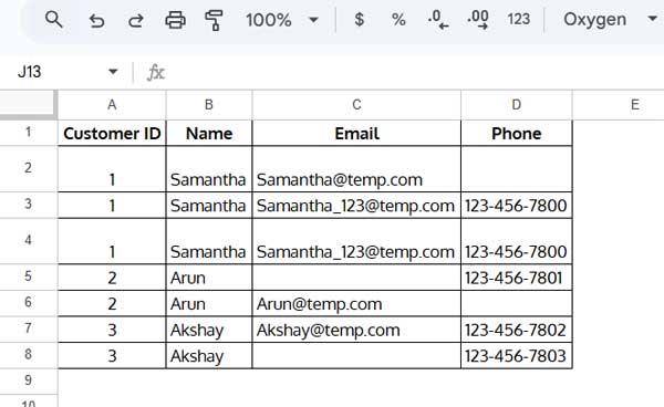
In this sample data, we will combine duplicate records based on Customer ID.
Steps to Combine Duplicate Rows in Google Sheets
Step 1: Extract Unique Customer IDs
Assume the sample data is in Sheet1. In Sheet2, enter the following formula in cell A1:
=TOCOL(UNIQUE(Sheet1!A1:A), 1)This will return the unique Customer ID values with the header:
| Customer ID |
| 1 |
| 2 |
| 3 |
Step 2: Combine Duplicate Records
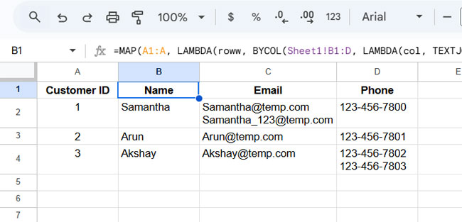
Now, in B1 of Sheet2, enter the following formula:
=MAP(A1:A, LAMBDA(roww, BYCOL(Sheet1!B1:D, LAMBDA(col, TEXTJOIN(CHAR(10), TRUE, UNIQUE(FILTER(col, Sheet1!A1:A=roww)))))))This formula consolidates duplicate records from Sheet1 into columns B to D in Sheet2.
Formula Explanation
If you haven’t already, open the sample sheet to follow along:
A1 Formula to Extract Unique IDs
=TOCOL(UNIQUE(Sheet1!A1:A), 1)- Extracts unique Customer IDs and removes empty cells.
B1 Formula to Combine Duplicate Rows
Here is a step-by-step explanation of the formula in B1.
FILTER(col, Sheet1!A1:A=roww)- Filters the current column (
col) in Sheet1!B1:D based on matching values in Customer ID (Sheet1!A1:A).
UNIQUE(...)- Removes duplicate values in the column.
TEXTJOIN(CHAR(10), TRUE, ...)- Joins the filtered results, separating them with a new line character (CHAR(10)).
Applying Across All Columns
- BYCOL ensures this logic is applied to each column (Name, Email, Phone) separately.
- MAP applies the logic to each unique Customer ID in A1:A.
Thus, the formula effectively combines duplicate rows in Google Sheets while preserving all necessary details.
Can you help me with my data? I have 4 columns, the first 3 have duplicates, and only the 4th column has different figures. I want to merge the duplicates and create a 4th column that is comma-separated. I checked out your other solutions using JOIN and FILTER, but I need to perform an array operation because I am importing the data from the IMPORTRANGE() function.
Hi Avishkar,
Sure. When I coded those formulas, the LAMBDA function was not available in Google Sheets.
That being said, I assume your sample data is in cells A1 to D and cells A1 to D1 contain the field labels IP, MAC, Hostname, and Anomaly.
Here is the code that you can try:
=LET(distinct,UNIQUE(A2:C),HSTACK(distinct,MAP(CHOOSECOLS(distinct,1),CHOOSECOLS(distinct,2),CHOOSECOLS(distinct,3),LAMBDA(ip,mac,host,
TEXTJOIN(", ",TRUE,FILTER(D2:D,A2:A&B2:B&C2:C=ip&mac&host))))))
I will try to post a custom function soon. Please watch for my upcoming post.
Thanks, Prashant for the guidance above, it is so close to what I’m trying to achieve! Instead of taking the MAX(), I just need the column data from the latest row. How can I do that please? Been trying for a couple of hours, thanks Prashant.
Hi, Junnie Chen,
To write a formula, I need more info like;
Do you want only the latest rows?
Do you have a timestamp column in your dataset?
Better, you may please share the URL of a sample of your sheet (after replacing confidential data with dummy data and removing personal info) via reply. The file should be in either View or Edit mode.
Thanks, Prashanth for getting back. Basically, there is a form for students to key in their exam marks, they could submit the form more than 1 time, so yes there will be Timestamp.
My goal is to show the summary of each student & their marks and grades in the “Subjects & Grades (Combined)” sheet. For each subject, I want to show the marks and grades from the latest row (as highlighted in orange in the “Subjects & Grades (ALL)” sheet). Currently, the formula I am using is showing the MAX() of marks and grade which is incorrect. Appreciate your guidance, thanks.
This is the sheet: …link removed by admin…
Hi, Junnie Chen,
I have created a new tab named “prashanth @infoinspired” in your shared Sheets.
In that, the main formula is in cell B2 which dragged down (not to right).
=ArrayFormula(IFERROR(REGEXEXTRACT(trim(query(filter(sort('Subjects & Grades (ALL)'!$B$2:$AC,row('Subjects & Grades (ALL)'!$A$2:$A),0),sort('Subjects & Grades (ALL)'!$A$2:$A,row('Subjects & Grades (ALL)'!$A$2:$A),0)=A2),,9^9)),"[A-Za-z0-9.]+")))
That’s the only formula you have to pay attention to.
Note:- The formula formats numbers to text. But you can use VALUE to convert in case you want to use it in aggregation.
I’ll write a tutorial later and will leave the link below.
Thank you for all of your helpful tutorials, I appreciate it.
I have some data where I am trying to use the formula in this tutorial to output a single row with title, color, size (qty).
I am having trouble joining all of the sizes to output in one line or in separate columns.
Currently, it is outputting the last size it encounters in column H. Any suggestions are much appreciated.
Hi, Kevin Watson,
It seems a pivot table is the best option to solve the problem. You can use the following Query Pivot.
=query(A1:D,"Select A,B,sum(D) where A is not null group by A,B pivot C",1)The above formula will return title in the first column, color in the second column, and summed quantities under various sizes from column 3 onwards.
The third column has no label as it represents “NIL” sizes. If you want to label it, use the below Query instead.
=query(query(A1:D,"Select A,B,sum(D) where A is not null group by A,B pivot C",1),"Select * label Col3'Nil'",1)Your sheet is view only. So I haven’t inserted the formula in your sheet.
Thank you for your help!
Thank you so much, this is perfect!
Thanks for this awesome query. Noticed some odd behavior. I’m using the query that looks for dups only in the first column.
Works beautifully as long as the entries in the first column are strings, not numbers. If the entries are numbers, it seems to drop some. Not sure if this is an issue with the query or Google Sheets.
But if you try it out with just for rows with two dups, it’ll work with strings in the first column: it returns two rows with the rest of the columns merged.
If you change the first column to numbers, it returns only one row, original one of the original rows.
Any ideas what’s causing this?
Hi, Erik,
Try formatting the numbers to Pure Text by selecting the column and then applying the required format from the menu Format > Number > Plain text.
If you don’t want to physically format the numbers to text, do it virtually using the To_Text function within Query.
Read: How to Use To_text Function in Google Sheets [Also the Use in Query].
Awesome, thank you–that worked. Still curious about why, but at least there’s a workaround! Cheers again!
Hello,
What if I’d like to combine rows in a way that I get two X where the same name has an X in the same column but on two different rows.
Is there a way to accomplish that?
Thanks
Andrea
Hi, Andrea,
The purpose of the above tutorial/formula is different.
Regarding your query, I think you may need to use a Filter combination formula to get your desired result. I have demonstrated the same in my Example tab named ‘User Query 2’. It’s not an Array Formula.
Best,
Hello Prashanth,
Thank you for your answer. I took a look at the example tab but maybe I didn’t fully explain myself.
Basically, concatenate the values if the name match and the same cell is filled.
Thank you again
Andrea
Hi, Andrea,
See if this new tutorial related to the same topic helps?
Merge Duplicate Rows in Google Sheets and Concatenate Values
Super it’s working. thanks for your nice and detailed help.
Hi there,
Thank you for this! Is there any way to not have the columns retitle with “Max”? Likewise, I’m getting an extra row added after the first row in the new array- is that supposed to happen and can I stop that from happening?
Thank you!
Hi, Kristen,
Actually, in my formula, the outer Query is to remove that titles. I don’t know why it’s not happening in your case.
If I can see a copy of your Sheet, of course after removing personal/confidential/sensitive data, I can suggest a solution.
Did you check my example sheet, that I have shared at the last part of my tutorial?
Best,
I am also having the word “max” added which makes the output uninterpretable.
This is so close to the perfect solution for me!
Here is my sheet: URL removed by admin
I would like to merge the duplicate rows in ‘alphatranspose’ tab in the separate ‘merge’ tab but without the “max” is added to one of the rows.
What am I doing wrong?
Thanks
Hi, Nick,
You have perfectly followed my instructions to merge duplicate rows. The issue is not from your side.
The Query function guesses the header row if you omit the header row (did not specify) number in the Query.
QUERY(data, query, [headers])In my second Query formula (the outer Query formula) I have omitted the header and leave the Query to guess it. In your case, the Query guessed the header row number as 1. Please specify it to 0 to avoid the max row.
You can do that by putting the value 0 just after the Offset clause in the second Query as below.
"Select * where Col1 is not null Offset 1",0)}I’ll update the formula in my post and my shared sheet also to incorporate the change.
Best,
Prashanth KV
Dammit, I should’ve worked THAT out! I was so close.
This is now working perfectly, thank you so much!
Thank you for your help Prashanth! This worked perfectly.
Is there any way to get the data to stop adding in alphabetical order and just append to the bottom of the list?
I have triggers set up for my data set, but somehow this formula formats A-Z and triggers all of my leads when a name like “Adam” gets appended to the top instead of the bottom of the list in chronological order.
Hi, Ellysha Chavez,
For this question, I may want to see the data. If possible, please prepare an example sheet (I only need some demo data) and share.
Thanks.
Thanks for responding!
Here is a Demo link. There are two tabs. The first tab is where the duplicate leads populate. The “Dedup” sheet is where the formula is and you can see they get formatted in alphabetical order. I don’t need them in alphabetical order, I need them to append to the bottom of the list when new leads populate.
— link removed by admin —
Also, seem to be having issues w/ Upper and lower case not combining duplicates because the last name may be “som” or “Som”.
Hi, Ellysha,
Thanks for sharing your example sheet. That helped me to well understand the problem.
I have made a copy of your shared sheet, I hope you don’t mind since it’s a demo sheet, and entered my solution there. I’ve just edited my post and at the end, shared your demo sheet with my solution entered in cell J1 (tab name: “User Question”).
Here is that formula.
={A1:I1;Query(ArrayFormula(query({A1:I},"Select upper(Col1),upper(Col2),Col3,lower(Col4),"&ArrayFormula(join(", ","Max(Col"&column(E1:I1)&")"))&"group by upper(Col1),upper(Col2),Col3,lower(Col4) order by Max(Col9)",1)),"Select * where Col1 is not null Offset 1",0)}In this, I have made the grouping columns, i.e. first name, last name and email address to upper/lower case letters. So it’ll solve the case sensitive problem.
To arrange the data based on your new leads, I have sorted the data based on your timestamp column.
Cheers!