This post explains how to fix interchanged first and last names in a running count array formula in Google Sheets.

A regular running count array formula will treat interchanged names as distinct entries, resulting in an incorrect count.

For example, if the name “Denise Young” appears twice and “Young Denise” appears thrice, the correct occurrence numbers should be {1, 2, 3, 4, 5}. However, the incorrect result would be {1, 2, 1, 2, 3}. Please see Figure 1 below for reference.

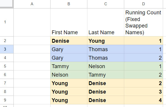
In this example, I have used an array formula in cell D2 to fix interchanged first and last names, ensuring the correct running count is returned.

Important Note:

One limitation of this formula is that it treats swapped names as identical. For instance, “Essie Phelps” and “Phelps Essie” will be counted as the same name, even if they are distinct entries. Keep this in mind when applying the solution.

How to Fix Interchanged First and Last Names in Running Count in Google Sheets

We will use a LAMBDA formula to return the correct running count while accounting for interchanged first and last names.

Here is the formula:

=ARRAYFORMULA(
   MAP(
        B2:B, 
        C2:C,
        LAMBDA(first, last, 
           IF(first & last = "", , SUM(COUNTIFS(B2:first & C2:last, {first & last, last & first})))
        )
   )
)

Formula Breakdown:

• B2:B: Range containing first names.
• C2:C: Range containing last names.
• B2 and C2: The starting cells of the respective ranges.

This is an array formula, so you only need to enter it in cell D2, and it will expand automatically. If there are values in the column that block the formula’s expansion, you may encounter a #REF! error.

How the Formula Works:

Let’s break down the formula step by step.

Step 1: Non-Array Formula to Fix Interchanged Names

To begin, we can use a non-array formula to handle interchanged names in the running count. The key is using the COUNTIFS function with an OR-like condition to check for both name orders.

Here’s the formula:

=ArrayFormula(
   SUM(
      COUNTIFS($B$2:B2 & $C$2:C2, {B2 & C2, C2 & B2})
   )
)

• Place this formula in cell D2 and drag it down to calculate the running count.

How It Works:

The COUNTIFS function counts occurrences of names in both orders:

=ArrayFormula(
   COUNTIFS($B$2:B2 & $C$2:C2, {B2 & C2, C2 & B2})
)

• Criteria Range: $B$2:B2 & $C$2:C2 combines first and last names.
• Criteria: {B2 & C2, C2 & B2} checks for both possible name orders.

The ARRAYFORMULA is required because, when dragging the formula down, the criteria range becomes an array. Combining two arrays using the ampersand (&) requires the use of the ARRAYFORMULA to handle the operation correctly.

The SUM function totals the results from the COUNTIFS function, ensuring a running count.

Step 2: Converting to an Array Formula

To avoid dragging the formula manually, we convert it into an array formula using the MAP function.

The syntax of the MAP function is:

MAP(array1, [array2, ...], LAMBDA)

• array1: B2:B (first names).
• array2: C2:C (last names).

We define placeholders (first and last) for the first and last names within the LAMBDA function:

=ARRAYFORMULA(
   MAP(
        B2:B, 
        C2:C,
        LAMBDA(first, last, 
           SUM(COUNTIFS(B2:first & C2:last, {first & last, last & first}))
        )
   )
)

Step 3: Handling Blank Cells

The above formula may inadvertently count blank cells. To prevent this, we wrap the formula with an IF condition to skip blank rows:

=ARRAYFORMULA(
   MAP(
        B2:B, 
        C2:C,
        LAMBDA(first, last, 
           IF(first & last = "", , SUM(COUNTIFS(B2:first & C2:last, {first & last, last & first})))
        )
   )
)

This ensures that the formula only processes rows with valid data.

Conclusion

This formula fixes interchanged first and last names in a running count. By using the MAP function and LAMBDA, we eliminate the need for manual adjustments, providing a dynamic and efficient solution.

Feel free to explore and adapt the formula to your specific needs!