Fix Fractional Percentage Formatting Issues in Google Sheets

Applying data validation is the only effective solution to resolve issues related to fractional percentage formatting in Google Sheets.

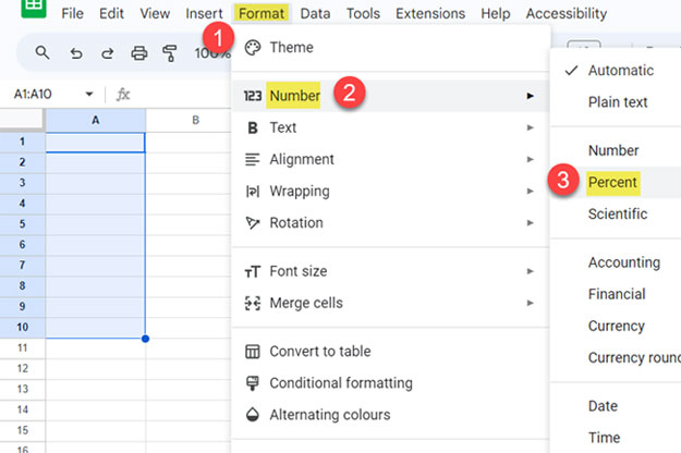
You can format a cell or range as a percentage by selecting the range and navigating to Format > Number > Percent.

For example, if you apply percentage formatting to the range A1:A10, you can enter 2.5 to display 2.5% and 0.75 to display 0.75%.

However, an issue arises when entering fractional percentages. If you enter .75 instead of 0.75, Google Sheets will display it as 0.75 (not 0.75%).

The solution is to restrict entering fractional percentages without the leading zero using data validation.

Here’s how to prevent percentage formatting issues when entering decimal percentages in Google Sheets.

Step 1: Apply Percentage Formatting

Apply the Percent formatting to the range A1:A10 (or any other range you choose). First, select the range A1:A10. Then click on Format > Number > Percent.

Example of percentage formatting in Google Sheets

To test the formatting, enter a value in the range. For example, enter 10 in cell A1, and it will be displayed as 10.00%.

Try entering a fractional percentage in cell A2, such as 0.5, which will be displayed as 0.50%.

Avoid entering .5 directly, as it will be formatted as 0.50 and will break the percentage formatting. If you do enter it, remember to apply Format > Number > Percent to that cell. Then proceed to the next step.

Step 2: Use Data Validation to Restrict Percentage Entry

Apply the following rule to the range A1:A10 to fix the fractional percentage formatting issue:

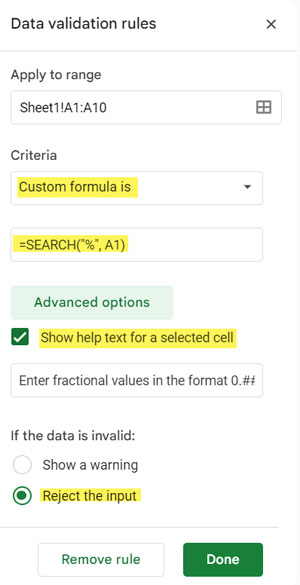
=SEARCH("%", A1)

If you apply this rule to a different range, replace A1 with the top-left cell of that range. For example, if applying to B2:E20, use B2.

To set up data validation for range A1:A10 to allow only percentage values like 0.5, 0.25, 10, etc., and to fix the fractional percentage issue, follow these steps:

Select A1:A10.
Click Data > Data Validation.
Click Add Rule.
Select “Custom formula is” under Criteria.
Copy and paste the formula above into the formula field.
Under Advanced Options, check “Show help text for selected cell”.
In the help text field, enter: “Enter fractional values in the format 0.##, not as .##.”
Check “Reject input”.
Click Done.

Data validation to reject fractional percentages like .5

Step 3: Test the Fix for Fractional Percentage Formatting

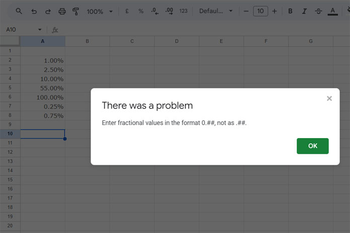
Now, when you enter values such as 1, 2.5, 10, 55, 100, 0.25, or 0.75, they will be converted to 1.00%, 2.50%, 10.00%, 55.00%, 100.00%, 0.25%, and 0.75% respectively.

However, if you try to enter .75, the sheet will reject the input with a warning: “Enter fractional values in the format 0.##, not as .##.”

Testing the fix for fractional percentage formatting in Sheets

This process resolves fractional percentage formatting issues in Google Sheets.

Resources

Here are some resources on percentage calculations in Google Sheets:

Case-Sensitive Running Count in Google Sheets