Learn how to efficiently find the first occurrence of specific weekdays, such as Sunday, Monday, and more, in any given month using Google Sheets.
Sometimes, you may need to identify the first occurrence of a specific weekday (Sunday, Monday, Tuesday, Wednesday, Thursday, Friday, or Saturday) in a given month using Google Sheets.
While you might already have a formula to find a particular weekday, adjusting it for a different weekday can be challenging.
I’ve created a dynamic formula that enables you to designate weekdays using week numbers (1 to 7, where 1 is Sunday and 7 is Saturday). This allows you to easily pinpoint the first occurrence of your desired weekday.
The formula streamlines the process by integrating the FILTER, SEQUENCE, and WEEKDAY functions.
Finding the First Sunday of a Given Month in Google Sheets
You have the flexibility to use different inputs: a month name, a month number, or the beginning of the month date. The formula adapts accordingly. I recommend using the beginning of the month date, involving both month and year. Let’s start with that, and I’ll guide you on adjustments for the month name or number.
For instance, to find the first Sunday date in January 2023:
- Enter 01/01/2023 in cell A1.
- To find the first Sunday of January, enter the following formula in cell A2:
=TO_DATE(
   FILTER(SEQUENCE(7, 1, A1), WEEKDAY(SEQUENCE(7, 1, A1))=1)
)
To locate the first Sunday of the current month, substitute A1 with EOMONTH(TODAY(), -1) + 1. In this context, the EOMONTH function converts today’s date into the end-of-the-month date of the previous month. +1 results in the beginning-of-the-month date for the current month.
Note:
In the above formula, we can avoid repeated calculations by using LET, thereby improving it. Here it is:
=LET(
  d, SEQUENCE(7, 1, A1),
  TO_DATE(
     FILTER(d, WEEKDAY(d)=1))
  )
Anatomy of the Formula
The aforementioned is essentially a FILTER formula. Here’s an explanation of how it works.
Syntax:
FILTER(range, condition1, [condition2, …])Where:
- range:
FILTER(SEQUENCE(7, 1, A1) - condition1:
WEEKDAY(SEQUENCE(7, 1, A1))=1
The SEQUENCE function generates a sequence of 7 dates, starting from the given date in cell A1, representing the beginning of the month.
The FILTER function then filters this sequence, selecting only the date where the weekday number is equal to 1 (Sunday).
The outcome is a date value, and the TO_DATE function is applied to format it back into a valid date.
How to Find First Monday, Tuesday, and Other Weekday Dates in Google Sheets
You now have a flexible formula to effortlessly find the first Sunday, Monday, etc., date in a month in Google Sheets.
To find the first Monday, simply replace the filter criterion ‘1’ with ‘2’:
=LET(
  d, SEQUENCE(7, 1, A1),
  TO_DATE(
     FILTER(d, WEEKDAY(d)=2))
  )
Here are the weekday numbers that you can use to find the first weekday of your choice:
| Day of the Week | Weekday No. |
| Sunday | 1 |
| Monday | 2 |
| Tuesday | 3 |
| Wednesday | 4 |
| Thursday | 5 |
| Friday | 6 |
| Saturday | 7 |
For example, to get the first Thursday in January 2024, follow these steps:
- Enter 01/01/2024 in cell A1.
- In cell A2, enter the following formula:
=LET(
  d, SEQUENCE(7, 1, A1),
  TO_DATE(
     FILTER(d, WEEKDAY(d)=5))
  )
Here, I’ve used the weekday number ‘5’ as the criterion.
Utilizing Month Text or Month Number Instead of Date in the Formula
In our examples, we’ve employed the beginning-of-the-month dates.
For instance, to locate the first Thursday in February 2023, instead of entering 01/02/2023, you can input either 2 or ‘February’ in cell A1.
- If you input 2 (the month number), replace A1 in the formula with
DATE(2023, A1, 1). - If you input ‘February’ (the month text), replace A1 in the formula with
DATE(2023, MONTH(A1&1), 1).
Locating the First Sunday, Monday, etc., Date in Every Month
In all of the above examples, we’ve used the formula to find the first Sunday, Monday, Tuesday, etc., of a particular month. What about every month in a year?
This is a bit tricky. We will use two additional functions: EDATE and MAP Lambda.
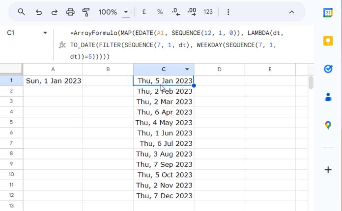
Let’s see how to get the first Thursday of every month in the year 2023.
=ArrayFormula(
  MAP(
  EDATE(A1, SEQUENCE(12, 1, 0)),
  LAMBDA(dt,
  TO_DATE(
       FILTER(SEQUENCE(7, 1, dt), WEEKDAY(SEQUENCE(7, 1, dt))=5)
  ))))
Anatomy of the Formula
Here are the steps to follow:
- Enter the date 01/01/2023, the year start date, in cell A1.
- Enter the following formula to get the first Thursday of 2023 in January in cell C1:
=TO_DATE(
   FILTER(SEQUENCE(7, 1, A1), WEEKDAY(SEQUENCE(7, 1, A1))=5)
)
Now, let’s use MAP with it:
=MAP(A1, LAMBDA(dt,
  TO_DATE(
      FILTER(SEQUENCE(7, 1, dt), WEEKDAY(SEQUENCE(7, 1, dt))=5)
)))
Syntax of the MAP Function:
MAP(array1, [array2, …], lambda)Where:
array1:A1lambda: The LAMBDA is as per the syntaxLAMBDA([name, …], formula_expression). Wherenameisdt, andformula_expressionisTO_DATE(FILTER(SEQUENCE(7, 1, dt), WEEKDAY(SEQUENCE(7, 1, dt))=5)).
The purpose of the MAP function is to return a new array formed by mapping each value in the given arrays to a new value, which is obtained by applying a lambda.
In the above example, we have a single value, not an array, which is A1.
To feed it an array that contains the beginning of the month dates for all months in 2023, i.e., the dates 01/01/2023, 01/02/2023, 01/03/2023, and so on, we can use the following EDATE formula to generate those dates:
ArrayFormula(EDATE(A1, SEQUENCE(12, 1, 0)))So, replace A1 in the MAP formula with this EDATE formula (you can move the ArrayFormula to the front):
=ArrayFormula(MAP(EDATE(A1, SEQUENCE(12, 1, 0)), LAMBDA(dt, TO_DATE(FILTER(SEQUENCE(7, 1, dt), WEEKDAY(SEQUENCE(7, 1, dt))=5)))))To get the first Sunday of every month in 2023, replace the filter criterion ‘5’ with ‘1’ as earlier.
That’s all for now. Thanks for staying. Enjoy!


This was so much help. Thanks!