Find the Last Row in Each Group in Google Sheets

You can use a simple SORT and SORTN combination to find (or extract) the last row in each group in Google Sheets. This method does not require a date column. Instead, it flips the data and removes duplicates based on a key column.

Example of extracting the last row in each group in Google Sheets using SORTN

Generic Formula

=SORTN(SORT(data, ROW(col)*LEN(col), FALSE), 9^9, 2, col_no, TRUE)

Where:

data – The range from which to extract the last row of each group.
col – The key column used to identify groups.
col_no – The column number of the key column in the dataset.

Example: Find the Last Row in Each Group in Google Sheets

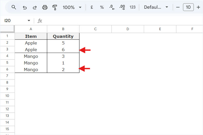
Consider the following dataset in A1:B, where column A contains fruit names, and column B contains quantities:

Item	Quantity
Apple	5
Apple	6
Mango	3
Mango	1
Mango	2

Formula to Extract the Last Row in Each Group

Enter the following formula in D2:

=SORTN(SORT(A2:B, ROW(A2:A)*LEN(A2:A), FALSE), 9^9, 2, 1, TRUE)

Expected Output:

Apple	6
Mango	2

How the Formula Works

SORT(A2:B, ROW(A2:A) * LEN(A2:A), FALSE) – This sorts the data by row numbers in descending order, effectively flipping the dataset.
- ROW(A2:A) * LEN(A2:A) – Creates a virtual helper column for sorting, using row numbers. Empty cells are ignored.
SORTN(..., 9^9, 2, 1, TRUE) –
- Extracts all rows (9^9 ensures all rows are considered).
- Removes duplicates based on column 1 (the key column).
- Returns the result sorted in ascending order.

Find the Last Row in Each Group Based on Multiple Columns

Sometimes, you may need to extract the last row in each group when grouping by multiple columns. Consider the following dataset in A1:C:

Item	Area	Quantity
Apple	North	5
Apple	South	4
Apple	South	2
Mango	West	3
Mango	East	1
Mango	West	4

Desired Output:

Apple	North	5
Apple	South	2
Mango	East	1
Mango	West	4

Formula to Find the Last Row in Each Group Based on Multiple Columns:

=SORTN(SORT(A2:C, ROW(A2:A)*LEN(A2:A), FALSE), 9^9, 2, 1, TRUE, 2, TRUE)

How This Works

The SORT function flips the dataset by sorting based on row numbers.
The SORTN function removes duplicates based on the first two columns, returning the last entry in each multi-column group.

Compared to the single-column grouping, the sorting performed in the SORTN is different. You can see that the sorting is performed in the first column (primary group) and the second column (secondary group), i.e., 1, TRUE, 2, TRUE.

Conclusion

Use the SORT + SORTN method to find the last row in each group in Google Sheets, even when a date column is unavailable. Instead of relying on timestamps, this formula flips the data and removes duplicates. If you have a date-based dataset, check out the resources below for alternative SORTN approaches.

Dear Prasanth,

Thank you for your great blogs, this helps a lot!

Would you maybe be able to assist me with the following query?

We use google sheets daily in our hotel to manage our minibar in all the hotel rooms. Each room has 3 products (actually more, but this is easier for the example below). Basically, we use google forms whenever we replace an item in a room, to keep track of the expiry date of all items in all rooms.

The sheet is structured as follows:

A B C D
Timestamp Room Item Expiry date of new item
04/07/2019 10:01:02 104 Product 1 15/03/2019

Each time a product is replaced in one of the rooms, a new line will be added to the Google Sheet. This means that the old entries will remain in the sheet (and actually become obsolete, because we replaced the product). We then use filter views to get the data we want.

However, for 1 particular thing, we do not manage the correct view/formula. What we like to do, is get a daily list of items which are expiring in the coming 10 days (so that we can replace them before they actually expire). I have already created a filtered view on the D column, however, the problem is that we always need to have the LATEST entry only for a certain product in a certain room, because the old rows will remain in the file over time.

So basically, I need to have a list first of each room with 3 unique products with the most recent time stamp for each (column A). It would look like this:

A B C D
Timestamp Room Item Expiry date of new item
4/07/2019 10:01 101 Product 1 25/03/2019
8/07/2019 11:31 101 Product 2 1/07/2019
29/06/2019 12:18 101 Product 3 25/03/2019
5/07/2019 11:24 102 Product 1 1/07/2019
9/07/2019 12:24 102 Product 2 29/01/2019
4/07/2019 10:01 102 Product 3 1/07/2019
8/07/2019 11:31 103 Product 1 25/03/2019
29/06/2019 12:18 103 Product 2 1/07/2019
5/07/2019 11:24 103 Product 3 29/01/2019

I could then apply the filter view mentioned before, on this list to get the list of items I want.

Hoping this makes sense? You would really be of great help if we can solve this.

Many thanks in advance.

Kind regards,
Max

7 COMMENTS

Desmond Lee October 21, 2022 At 5:36 am

Thank you

Desmond Lee October 20, 2022 At 9:27 am

Hi Prashanth

I have a question here.

How do I extract the last row of “Apple” by the latest timestamp in an unsorted table? Let’s say;

24-Apr 2018 09:00:21 Apple
22-Apr 2018 16:08:43 Apple
24-Apr 2018 09:00:21 Orange
24-Apr 2018 15:00:09 Apple
22-Apr 2018 08:00:21 Apple

Answer : 24-Apr 2018 15:00:09 Apple

- Prashanth October 20, 2022 At 3:51 pm
  
  Hi, Desmond Lee,
  
  Assume the above table range is A1:B, where column A contains timestamps and column B contains the fruit names.
  
  So the formula you may use is –
  
  =index(sort(filter(A:B,B:B="Apple"),1,0,2,1),1,0)
  
  The formula may convert the timestamp to a datevalue. So format it back to timestamp (Format > Number > Date time).
  
  To get all fruits (latest).
  
  =sortn(sort(A:B,1,0,2,1),9^9,2,2,1)
  
Max July 10, 2019 At 8:09 am

Dear Prasanth,

Thank you for your great blogs, this helps a lot!

Would you maybe be able to assist me with the following query?

We use google sheets daily in our hotel to manage our minibar in all the hotel rooms. Each room has 3 products (actually more, but this is easier for the example below). Basically, we use google forms whenever we replace an item in a room, to keep track of the expiry date of all items in all rooms.

The sheet is structured as follows:

A B C D
Timestamp Room Item Expiry date of new item
04/07/2019 10:01:02 104 Product 1 15/03/2019

Each time a product is replaced in one of the rooms, a new line will be added to the Google Sheet. This means that the old entries will remain in the sheet (and actually become obsolete, because we replaced the product). We then use filter views to get the data we want.

However, for 1 particular thing, we do not manage the correct view/formula. What we like to do, is get a daily list of items which are expiring in the coming 10 days (so that we can replace them before they actually expire). I have already created a filtered view on the D column, however, the problem is that we always need to have the LATEST entry only for a certain product in a certain room, because the old rows will remain in the file over time.

So basically, I need to have a list first of each room with 3 unique products with the most recent time stamp for each (column A). It would look like this:

A B C D
Timestamp Room Item Expiry date of new item
4/07/2019 10:01 101 Product 1 25/03/2019
8/07/2019 11:31 101 Product 2 1/07/2019
29/06/2019 12:18 101 Product 3 25/03/2019
5/07/2019 11:24 102 Product 1 1/07/2019
9/07/2019 12:24 102 Product 2 29/01/2019
4/07/2019 10:01 102 Product 3 1/07/2019
8/07/2019 11:31 103 Product 1 25/03/2019
29/06/2019 12:18 103 Product 2 1/07/2019
5/07/2019 11:24 103 Product 3 29/01/2019

I could then apply the filter view mentioned before, on this list to get the list of items I want.

Hoping this makes sense? You would really be of great help if we can solve this.

Many thanks in advance.

Kind regards,
Max

- Prashanth July 10, 2019 At 6:42 pm
  
  Hi, Max,
  
  Assume the above data is in A1:D in “Sheet1” (A1:D1 contain the headers).
  
  If you are ready to manually sort this data (the timestamp column) in descending order, then you can use the below formula in the same sheet (in cell F2). The formula will return the ‘recent’ unique three products in each room.
  
  =sort(sortn(A2:D,9^9,2,B2:B&C2:C,0),2,1,3,1)
  
  If you are not ready to sort the data, then in “Sheet2”, sort the data using the below formula in cell A2.
  
  =sort(Sheet1!A2:D,1,0)
  
  Then in cell F2 in “Sheet2” use the first formula.
  
  Best,
  
Rekha April 29, 2019 At 3:31 am

Prasanth, Thank you for the wonderful tutorial.

Your formula is giving the full total last row, but I only want to add a column next to G, i.e in column H I would like to get the last value that is in column G. How should I get this?

Can you please advise?

Thank you.

Rekha

- Prashanth April 29, 2019 At 10:36 am
  
  Hi, Rekha,
  
  First, modify the earlier formula as below.
  
  =sortn(sort({if(len(A2:A),row(A2:A),""),A2:G},1,false),9^9,2,4,false)
  
  Here are the changes made:
  
  1. Removed the ArrayConstrain (earlier used to remove the virtual column that contains the row numbers).
  2. Removed the ArrayFormula. When using SORT, ArrayFormula is not required. In earlier formula also, it’s not necessary to use.
  3. Moved the row number virtual column from the last to the first.
  
  Now in the next step, we can use this formula as the range in a Vlookup. So the final formula that you can use in cell H2 is;
  
  FINAL FORMULA (cell H2)
  
  =ArrayFormula(IFERROR(vlookup(row(A2:A),sortn(sort({if(len(A2:A), row(A2:A),""),A2:G},1,false),9^9,2,4,false),8,0)))
  
  The index number 8 indicates column G (see the last part of the formula). If you want to extract the values from any other column, just change that number accordingly.
  
  Best,