


")


")

")
")
 in Excel & Google Sheets")


How do I filter a range that contains a date of birth column for birthdays that fall in the next 30 days or the next ‘n’ days in Google Sheets?
To filter a range for upcoming birthdays, we can use the FILTER function along with various date functions in Google Sheets.
For this example, we will use the following sample data which contains names in A1:A and dates of birth in B1:B.
| Name | Birthday |
| Nicole Hill | 14/06/1991 |
| Jane Smith | 21/07/1985 |
| Anne Wood | 30/05/1991 |
| Terry Clark | 14/11/1979 |
| Carol White | 12/12/1990 |
Step 1: Converting Birthdays to This Year’s Birthdays
The following array formula will convert the birthdays to this year’s birthdays:
=ArrayFormula(
   LET(
      new_dt, DATE(YEAR(TODAY()), MONTH(DATEVALUE(B2:B)), DAY(B2:B)),
      IFERROR(IF(new_dt<TODAY(), EDATE(new_dt, 12), new_dt))
   )
)
You can enter it in cell C2, provided C2:C is blank. Then select C2:C and click Format > Number > Date to apply the date formatting.
This formula is critical for filtering upcoming birthdays in Google Sheets, so it’s worth taking the time to understand its core functionality.
How does this formula work?
The formula uses the DATE function to transform birthdays into dates for the current year.
Syntax:
DATE(year, month, day)Here’s the relevant part of the formula defined as new_dt using the LET function:
DATE(YEAR(TODAY()), MONTH(DATEVALUE(B2:B)), DAY(B2:B))year:YEAR(TODAY())— Extracts the current year from today’s date.month:MONTH(DATEVALUE(B2:B))— Extracts the month from the birthdays.- The DATEVALUE function ensures blank cells return errors, preventing MONTH from mistakenly interpreting them as December (#12).
day:DAY(B2:B)— Extracts the day from the birthdays.
This process converts each birthday into a date for the current year.
Handling Past Dates
Once converted, some birthdays may fall before today’s date. These need to be shifted to the next year. The following logical test addresses that:
IFERROR(IF(new_dt < TODAY(), EDATE(new_dt, 12), new_dt))IF(new_dt < TODAY()): Checks ifnew_dtis earlier than today.EDATE(new_dt, 12): IfTRUE, shifts the date 12 months forward (to next year).new_dt: IfFALSE, retains the date as is.
The IFERROR function handles any potential errors, while the ArrayFormula ensures the formula processes the entire range at once.
Step 2: Checking if This Year’s Birthdays Fall Within N Days
We want to filter the upcoming birthdays that fall within 30 days. So here, ‘n’ is 30.
Enter the following formula in cell D2 to return TRUE or FALSE Boolean values. TRUE means the birthdays fall within 30 days; FALSE means they do not.
=ArrayFormula(IF(C2:C="",,ISBETWEEN(C2:C, TODAY(), TODAY()+30, FALSE)))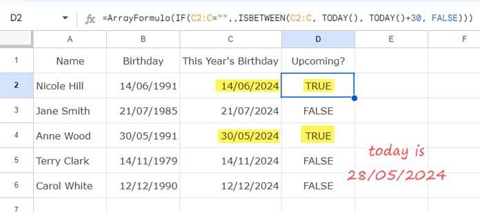
You should remove FALSE in the formula if you want to include today’s date when counting forward for upcoming birthdays. The current formula excludes today’s date in the count.
To filter upcoming birthdays that fall within the next week, replace +30 in the formula with +7.
The core part of this test is the ISBETWEEN function, and the syntax of this function is as follows:
ISBETWEEN(value_to_compare, lower_value, upper_value, [lower_value_is_inclusive], [upper_value_is_inclusive])Where:
value_to_compare: C2:C – This year’s birthdays.lower_value: TODAY() – today’s date.upper_value: TODAY()+30 – today’s date plus 30 days.lower_value_is_inclusive: FALSE.
The ISBETWEEN function returns TRUE for the dates that fall between today’s date and today’s date plus 30 (inclusive).
Step 3: Filtering for Upcoming Birthdays
We are in the final step. You just need to filter the range using a condition. Let’s move on to that formula.
=FILTER(A2:B, D2:D)The formula adheres to the syntax FILTER(range, condition1, [condition2, …]).
The formula returns the rows wherever D2:D contains TRUE.
This way, we can filter data by upcoming birthdays in Google Sheets.
If you want to avoid using helper columns, delete the formulas in C2 and D2 and use the following formula directly:
=ArrayFormula(
   LET(
      new_dt, DATE(YEAR(TODAY()), MONTH(DATEVALUE(B2:B)), DAY(B2:B)),
      ftr, IFERROR(IF(new_dt<TODAY(), EDATE(new_dt, 12), new_dt)),
      FILTER(A2:B, ISBETWEEN(ftr, TODAY(), TODAY()+30, FALSE))
   )
)