")
")


")


")

")
")
 in Excel & Google Sheets")


How do you filter one array using another array in Google Sheets? That’s the core of this tutorial — how to filter out matching keywords in Google Sheets, whether they are exact or partial matches. For this, you can choose between QUERY and FILTER. I prefer using the FILTER function — it’s simpler and more flexible.
This guide is about advanced keyword filtering using Google Sheets, a popular tool among content creators and SEOs. Let’s first understand the scenario.
In my Sheet, column A contains a long list of keywords. In column C, I have another list of keywords. For clarity, let’s call the keywords in column A total_keywords and those in column C used_keywords.
The goal is to create a formula in cell E1 that returns only the keywords from column A that do not appear in column C — either partially or fully.
Partial Match vs Full/Exact Match in Google Sheets
Let’s say you have the keyword “natural beauty tips” in column A (total_keywords) and “beauty” in column C (used_keywords). This is a partial match, and we want to remove such results from the final filtered output.
On the other hand, for an exact match, the formula should only exclude keywords in column A if they are an exact copy of any keyword in column C. In that case, “natural beauty tips” stays because it’s not exactly “beauty.”
In this tutorial, you’ll learn how to filter out matching keywords in Google Sheets, both fully and partially. If you’re looking for the opposite use case — filtering values that do match — check out my guide on Filter Based on a List in Another Tab in Google Sheets. You can also adapt the same formulas here by changing the Boolean flag FALSE to TRUE.
How to Filter Out Partial Matching Keywords in Google Sheets
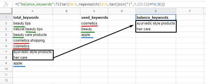
Here’s a screenshot showing the setup. In this case, column E contains the filtered results from column A, excluding any partial keyword matches found in column C.
Formula:
={"balance_keywords"; FILTER(A2:A, REGEXMATCH(LOWER(A2:A), TEXTJOIN("|", 1, LOWER(C2:C))) = FALSE)}Explanation:
We’re using the FILTER function to return only the rows from A2:A that do not partially match any of the keywords in C2:C.
Let’s break it down:
LOWER(A2:A): Converts all text in Column A to lowercase to make the comparison case-insensitive.LOWER(C2:C): Ensures that all the keywords in Column C are also lowercase for a fair match.TEXTJOIN("|", 1, LOWER(C2:C)): Joins the list of used keywords with a pipe (|) separator to create a regular expression pattern. This pattern is used to check if any of the keywords appear in each cell.- Example output:
"beauty|cosmetics|apple"
- Example output:
REGEXMATCH(...): Checks if any of the keywords in the pattern appear anywhere within each text inA2:A.= FALSE: This flips the logic — instead of keeping matches, we filter them out (i.e., we return only rows that don’t match any of the keywords).
How to Filter Out Fully Matching Keywords in Google Sheets
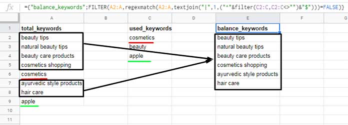
This formula filters out only those keywords that are exact matches with the list in column C.
Formula:
={"balance_keywords"; FILTER(A2:A, REGEXMATCH(LOWER(A2:A), TEXTJOIN("|", 1, ("^" & LOWER(TOCOL(C2:C, 3)) & "$"))) = FALSE)}Explanation:
^and$are used to ensure full matches (start to end).- For example:
^cosmetics$|^beauty$|^apple$ TOCOL(C2:C, 3)removes blank cells that could otherwise create issues like^$.
This pattern ensures that only fully matching keywords are removed. It avoids partial match problems like removing “natural beauty tips” just because “beauty” exists in the used list.
Note: If you skip the TOCOL around column C, the formula might pick up blank rows, causing incorrect regex like ^$.
Final Thoughts
Using these techniques, you can filter out matching keywords in Google Sheets precisely the way you need — partial or full match. It’s incredibly useful for SEO tasks like content audits, duplicate detection, or cleaning keyword lists.
Let me know in the comments if you face any issues or need a variation of this formula.