If you’re a content creator, marketer, or SEO specialist, you may want to extract listed keywords from existing titles as part of your workflow. With Google Sheets, this is easy — just keep your titles in one column and your list of focus keywords in another. A simple formula will scan each title and return the matching keywords (including combinations) in the corresponding row.
There’s no built-in function for this, but we can achieve it using a combination of TEXTJOIN, FILTER, REGEXMATCH, and LOWER.
In this tutorial, you’ll learn how to extract one or more keywords — even multi-word ones like “apple pie” or “banana smoothie” — from titles using a flexible formula. This is a practical method for anyone wondering how to extract listed keywords from titles in Google Sheets effectively.
Why Extracting Keywords from Titles Matters
Let’s look at this from a content creator’s perspective.
Identify Keyword Usage in Your Titles
- Instantly check if your post titles include target SEO keywords.
- Ensures your content is aligned with your keyword strategy.
Content Audit & Optimization
- Easily audit a large list of titles to find which keywords are used — and which are missing.
- Useful for updating or planning content around underused keywords.
SEO Reporting
- Create simple, structured reports that show which keywords appear in which titles.
- Helps you track keyword coverage across your content.
Tagging or Categorization
- Automatically assign content tags based on detected keywords.
- Helpful when organizing blog posts, videos, or podcast episodes in bulk.
Scale Content Research
- Analyze competitor titles to identify keyword gaps.
- Discover new opportunities in your niche based on what’s trending.
Use Case Example
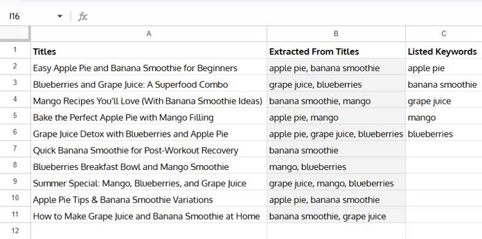
Let’s say you have a list of titles in column A:
Easy Apple Pie and Banana Smoothie for Beginners
Blueberries and Grape Juice: A Superfood Combo
Mango Recipes You’ll Love (With Banana Smoothie Ideas)
Bake the Perfect Apple Pie with Mango Filling
Grape Juice Detox with Blueberries and Apple Pie
Quick Banana Smoothie for Post-Workout Recovery
Blueberries Breakfast Bowl and Mango Smoothie
Summer Special: Mango, Blueberries, and Grape Juice
Apple Pie Tips & Banana Smoothie Variations
How to Make Grape Juice and Banana Smoothie at Home
And in column C, your list of target keywords:
apple pie
banana smoothie
grape juice
mango
blueberries
You want to extract listed keywords from column A titles using the list in column C.
The Formula to Extract Listed Keywords from Titles
Paste this formula in cell B2 and drag it down:
=TEXTJOIN(", ", TRUE,
   FILTER($C$2:$C$6,
      REGEXMATCH(LOWER(A2), "\b" & LOWER($C$2:$C$6) & "\b")
   )
)
Explanation:
REGEXMATCH(..., "\b" & keyword & "\b")ensures full word/phrase matching.LOWER()handles case-insensitive comparisons.FILTER()pulls out only the matching keywords.TEXTJOIN()combines multiple matches into a single cell, separated by commas.
This is one of the simplest yet most powerful ways to extract listed keywords from titles in Google Sheets — even when those keywords have spaces.
Want It to Spill Automatically?
If you’d like the formula to automatically process all titles in column A without dragging, use this version with MAP and LAMBDA:
=IFNA(
   MAP(A2:A, LAMBDA(row,
      TEXTJOIN(", ", TRUE,
         FILTER(D2:D6,
            REGEXMATCH(LOWER(row), "\b" & LOWER(D2:D6) & "\b")
         )
      )
   ))
)
Place it in B2, and ensure the rest of column B is empty so the formula can spill down.
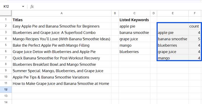
Summarize Keyword Matches Across Titles
Want to know how often each keyword appears? You can use QUERY to generate a frequency summary.
Since the earlier formula combines keywords with commas, you’ll first need to remove TEXTJOIN and convert results to a single column:
=QUERY(
   TOCOL(
      IFNA(
         MAP(A2:A, LAMBDA(row,
            TOROW(FILTER(C2:C6,
               REGEXMATCH(LOWER(row), "\b" & LOWER(C2:C6) & "\b")
            ))
         ))
      ), 3
   ), "select Col1, count(Col1) group by Col1"
)
This outputs a summary table showing how often each keyword appears across your list of titles.
Conclusion
If you’ve ever needed a scalable way to analyze and extract keywords from titles, now you know how to extract listed keywords from titles in Google Sheets using formulas. It’s flexible, fully customizable, and supports multi-word keyword matching. Whether you’re planning new content, auditing SEO, or tracking keyword usage, this approach will save time and deliver accurate results.


Update:-
If your keyword string list is more than 255 bytes, then the regex function fails.
Therefore if you simply limit each keyword list to 255 bytes and then use a new column for the overflow, then you concatenate results, everything does work.
Hi, todd furubayashi,
Thanks for your feedback!
Hello, the formula works great, but I am getting false positives for phantom matches.
My title data may be lengthy, but nothing is more than 255 bytes.
Is there a threshold where one may not want to risk using google sheets due to errors?
Thank you. The walking through of each formula module was a work of art.