Google Sheets Pivot table has two built-in options to filter the result table: Filter by values and Filter by condition. The former allows you to check or uncheck values to exclude or include. We are talking about the latter option.
Do you know how to filter multiple values in the Pivot table “Filter by condition” in Google Sheets? There are two methods.
- Experts recommend filtering the source data using Query or Filter before creating the Pivot table to filter out or filter in multiple values in the Pivot output. Use Query or Filter to extract the required values, then use this as the Pivot table source.
- Even though the above is a better option for filtering multiple values in the Pivot table, there is one more option. That’s using a custom Formula in the Filters field in the Pivot table editor.
To filter multiple values in the Pivot table in Google Sheets, you can use a custom formula within the Pivot editor panel in Google Sheets. I’ll come to that later. First, understand how to use Filters in the Pivot table editor.
Filter Pivot Table Data (Part of Pivot Customization)
Filtering data is one of the customization features in the Pivot table in Google Sheets.
On the Pivot table panel, there is a dedicated option named Filters > Filter by condition which contains several built-in filter commands like;
- Text contains.
- Text does not contain.
- Is equal to.
- Is not equal to.
- Text starts with.
- Text ends with, etc.
In addition to that, you can see a custom formula option and a subsequent field in the Pivot table filter.
You will get these once you add a field to Filters and choose the status Filter by condition.
The problem with these built-in Pivot table commands, except the custom formula, is it does not accept multiple values.
For example, you can’t use multiple values in Text contains or Text does not contain. Below you can see one Pivot example that demonstrates this shortfall.
Sample Data and Pivot Table to Filter by Text Does Not Contain
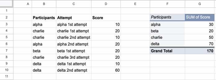
As you can see below, the source data is in the B2:D10 range. Our Pivot table from this source is created (Insert menu > Pivot table) in cell F2 (in the range F2:G7) in the same Sheet.

From this Pivot table report, I want to exclude the rows that contain “2nd” or “3rd” in the “Attempt” field. For your info, I haven’t used the said field in creating the Pivot table.
How to do that?
Using the built-in “Text does not contain” command in the Pivot table Filters, you can only exclude rows with strings “2nd” or “3rd,” not both.
See how to do that single value filter using “Text does not contain.”
I know most of you are already familiar with this. I am including it for newbies.
Steps:
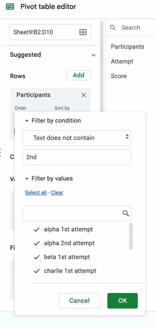
Click on the “Filters” option on the Pivot table editor panel, click “Add” and choose the field “Attempt.”
Then choose “Filter by condition” and under it, select “Text does not contain.”
Enter the value “2nd” and click OK. You can refer to the below image.

How to include multiple values in the “Text does not contain” then?
As mentioned at the beginning of this Google Sheets tutorial, we can depend on the custom formula field in the Pivot table Filters.
You can use a Regexmatch-oriented custom formula to filter multiple values in a Pivot table in Google Sheets.
Filter Multiple Values in Pivot Table Using Regexmatch in Google Sheets
Multiple Values in Text Does Not Contain
To exclude the rows that contain the values “2nd” or “3rd” (both), use the below Regexmatch in the Pivot table Filters custom formula field.
=REGEXMATCH(Attempt, "2nd|3rd")=FALSE // This is case sensitive
=REGEXMATCH(Attempt, "(?i)2nd|3rd")=FALSE // This is case in-sensitive
If you want, you can replace the field name “Attempt” with the range reference C3:C10.
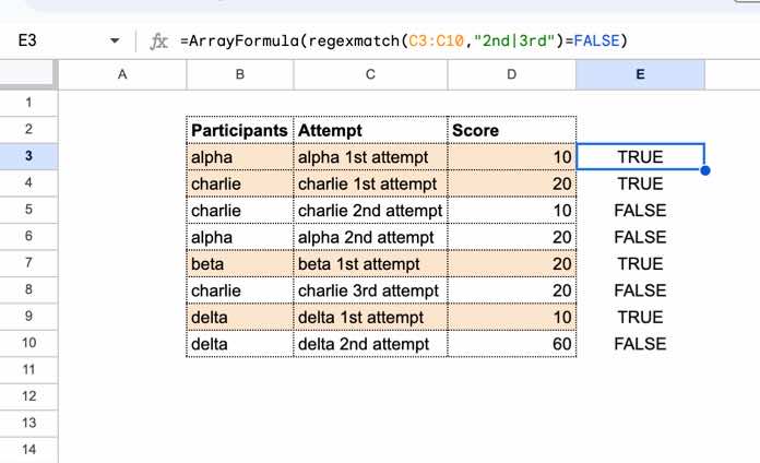
=REGEXMATCH(C3:C10, "2nd|3rd")=FALSEDo you know how this Regexmatch works within the Pivot table Filter? Please check this image.

I have entered one Regexmatch formula in cell E3.
It is different from the formula we used in the Pivot table Filters.
You must take care of two things when you enter Regexmatch outside the Pivot table editor.
- Include the ArrayFormula with Regexmatch as the reference C3:C10 is an array, not a single cell like C3. But not required within the Pivot table editor.
- Do not use the field name “Attempt” instead of C3:C10. The field names will only work within the Pivot table editor.
The Regexmatch returns TRUE if it matches “2nd” or “3rd”.
We require the FALSE part since we want multiple values in the “Text does not contain.”
That is why I have used =FALSE at the end of the Regexmatch formula.
Do you want to exclude more values?
Please follow the syntax =REGEXMATCH(C3:C10, "2nd|3rd|4th|5th")=FALSE.
Multiple Values in the Text Contains
To only include the values you want in the Pivot table, use the Regexmatch formula as below.
Please note that the following formula is similar to multiple values Does Not Contain. Here instead of =FALSE, we must use =TRUE.
=REGEXMATCH(Attempt, "2nd|3rd")=TRUEI hope you have enjoyed the above Pivot table customization tips.


Thank you for the tutorial. In your example, the field name is one word (i.e., “Attempt”). How do you address it when you have multiple words for the field name, for instance, “Material name” or “Number of units”? Range reference did not work for me. Thanks.
Specify them within single quotes.
E.g.:
=REGEXMATCH('All Attempts',"2nd|3rd")=FALSEHi Prashanth,
This is very helpful for me as well – many thanks.
i) I have to use a syntax with “;” instead of “,”, maybe because the sheet settings are “Locale = France” (this might address the remark made by nomwoyi Kunde on March 18, 2022).
ii) To EXCLUDE “2nd” and “3rd” attempts in the Pivot Table, I have to use the “FALSE” results of the regex (Filter applied to the “Attempt” column), i.e.:
=regexmatch(Attempt; "2nd|3rd") = FALSEIt works like a charm!
Best regards,
Thanks for your feedback.
Hello,
I’m following all the steps to use the custom filter, but it isn’t working.
Does the datasheet and pivot table have to be on the same page?
Hi, Enomwoyi Kunde,
Nope! Please check again. Also, you can leave the URL below (I will keep it unpublished)
Hi Prashanth,
This is very helpful – thanks.
Is there a way I can combine True and False in the same regexmatch formula? e.g. include “software” and exclude “SDR”
Thanks.
Ami
Hi, Ami Shimkin,
I may require an example to know what you are trying to do. From your question, I think FILTER may help.
Please feel free to share an example sheet link in the “Reply”.
Thanx for the reply. In my case, the data is on a different sheet so this won’t work.
I understand as of now it is probably not possible even with a script as filter views are not called through scripts.
I have already put a feature request many a time but so far it is not implemented.
But thanx anyway.
And you are really doing a good job.
I follow your post very diligently and find them very informative. I use the pivot table very extensively in my work.
I request if you can develop some script / some roundabout method to drill down to the filtered source data directly from the pivot table it would be a great help.
Presently the native feature creates a new sheet that is not of much use.
Hi, Srivastava,
Thanks for your feedback!
The similar thing you can achieve via Sheets’ new SLICERs. You can find that under the Data menu.
If your source data and the Pivot table are with in the same Sheet (same tab), you can filter your data and Pivot Table using this tool.
If the source and the Pivot table are in two different tabs, it won’t.
How to Use Slicer in Google Sheets to Filter Charts and Tables.
Here is one more related post – Drill Down Detail in Pivot Table in Google Sheets [Date Grouping]
Best,