You can filter a dataset by month and year using the QUERY function or the FILTER function in Google Sheets. I prefer the QUERY function as it retains the header row in the result.

To filter by month and year, we will use the MONTH and YEAR scalar functions in the WHERE clause of the QUERY function.

Before we proceed, it’s important to understand how to specify a condition in a date column, as QUERY uses a query string. Specifying criteria is not the same as with other native Sheets functions you might be familiar with. By “query string,” I mean the actual query to be executed.

Introduction

When specifying a date condition in the query, use the keyword DATE, followed by a string literal in the ISO 8601 date format (yyyy-mm-dd).

For example, if the date is 29th November 2024, it should be written as DATE '2024-11-29' when hardcoding. If the date is in cell A1, you should convert it to text in the ISO format using the Long-winded Approach or the compact form as follows:

'"&TEXT(H1, "YYYY-MM-DD")&"'

I prefer the compact method, as it is widely used and easier to follow.

Now that we’ve covered these basics, let’s proceed with filtering by month and year using the QUERY function.

Examples: Filter by Month and Year Using Query

Here’s the sample data:

Column A contains dates of purchase, column B contains pencil grades (either B for black or H for hard), and column C contains the purchase quantity. The first row is the header.

We will start by filtering by date, then by month, year, and finally by both month and year.

1. Filter by Date Duration in QUERY

The following two formulas will filter the sample data based on the dates in Column A.

In the first formula, we will enter the date directly within the formula:

=QUERY(A1:C,"SELECT * WHERE A >= DATE '2018-01-01' AND A <= DATE '2018-01-31'",1)

This filters the rows where the date in Column A falls between 1st January 2018 and 31st January 2018.

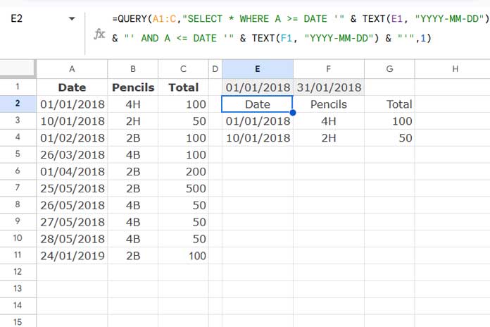
Alternatively, you can enter the date conditions in E1 and F1 and use the following formula:

=QUERY(A1:C,"SELECT * WHERE A >= DATE '" & TEXT(E1, "YYYY-MM-DD") & "' AND A <= DATE '" & TEXT(F1, "YYYY-MM-DD") & "'",1)

2. Filter by Month Using the MONTH Scalar Function in QUERY

The QUERY formula uses month numbers from 0 to 11, where 0 represents January and 11 represents December.

The following formula will filter the rows matching month number 0 (January) in column A:

=QUERY(A1:C,"SELECT * WHERE MONTH(A) = 0",1)

Alternatively, you can enter the month number (0 for January) in any cell, for example E1, and use the following formula:

=QUERY(A1:C,"SELECT * WHERE MONTH(A) = "&E1&"",1)

3. Filter by Year Using the YEAR Scalar Function in QUERY

The following QUERY formula will filter all records for the year 2018:

=QUERY(A1:C,"SELECT * WHERE YEAR(A) = 2018",1)

Alternatively, you can enter the year (2018) in any cell, for example F1, and use the following formula:

=QUERY(A1:C,"SELECT * WHERE YEAR(A) = "&F1&"",1)

4. Filter by Month and Year Using the QUERY Function

Filtering by both month and year is useful when you have data spanning multiple years. If you use only the MONTH function, you might get records from the same month across different years. So, it’s important to specify both the month and year.

Here’s the formula to filter by both month and year:

=QUERY(A1:C,"SELECT * WHERE MONTH(A) = 0 AND YEAR(A) = 2018",1)

This filters all records from January 2018.

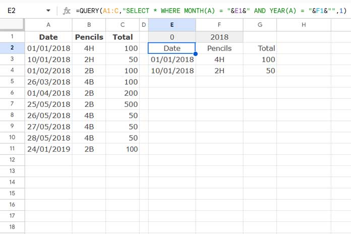
Alternatively, you can enter the month (0) in E1 and the year (2018) in F1, and use the following formula:

=QUERY(A1:C,"SELECT * WHERE MONTH(A) = "&E1&" AND YEAR(A) = "&F1&"",1)

Resources

• Creating Month-Wise Summary in Google Sheets (Query Formula)
• How to Use the MONTH Function in Google Sheets Query
• Query to Create Daily/Weekly/Monthly/Quarterly/Yearly Report Summary in Google Sheets
• Month Name as the Criterion in Date Column in Query Function in Google Sheets
• Sum Current Month Data Using the Query Function in Google Sheets
• Google Sheets Query to Extract All the Rows from the Previous Month
• How to Filter by Month in Google Sheets
• Filter by Upcoming Birthdays in Google Sheets