Google Sheets provides several methods for extracting usernames from single or multiple email addresses. You can use REGEXREPLACE, REGEXEXTRACT, LEFT+SEARCH, or SPLIT+CHOOSECOLS. We will discuss all these options below.
An email address, or email ID, has three parts: the first part is the username or local_part, followed by the “@” symbol, and finally the domain.
Whichever formula you choose to extract the username from the email address, you need to consider the “@” symbol, the second part of the email address. Because the username is the part before this symbol.
Formulas for Extracting Usernames from Email Addresses in Google Sheets
Assume cell A1 contains an email address. You can use any of the following formulas in another cell to extract the username:
REGEXREPLACE:
=REGEXREPLACE(A1, "@(.*)", "")This REGEXREPLACE formula matches the “@” symbol followed by any characters (zero or more) until the end of the string and replaces that part with an empty string, leaving only the username.
REGEXEXTRACT:
=REGEXEXTRACT(A1, "([^@]+)")This formula matches one or more characters that are not the “@” symbol. Since REGEXEXTRACT extracts the first matching occurrence, it returns only the username, not the domain.
LEFT + SEARCH:
=LEFT(A1, SEARCH("@", A1)-1)The SEARCH function finds the position of the “@” in the string. LEFT extracts characters from the beginning of the email address up to the position of “@” minus one, which gives the username.
SPLIT + CHOOSECOLS:
=CHOOSECOLS(SPLIT(A1, "@"), 1)The SPLIT function divides the email address at the “@” character, and CHOOSECOLS returns the first column of the result, which is the username.
Step-by-Step Guide
The username part of email addresses can contain alphanumeric characters and special characters such as periods, underscores, hyphens, plus signs, and percent signs.
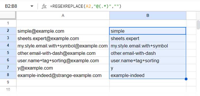
Consider the following sample email addresses in column A (range A2:A):
| simple@example.com |
| sheets.expert@example.com |
| my.style.email.with+symbol@example.com |
| other.email-with-dash@example.com |
| user.name+tag+sorting@example.com |
| y@example.com |
| example-indeed@strange-example.com |
To extract usernames from these addresses, enter one of the above formulas in cell B2. For example, using REGEXREPLACE:
=REGEXREPLACE(A2, "@(.*)", "")This formula will display the username in cell B2. Then, drag the fill handle from B2 down as far as needed to apply the formula to the rest of the cells.

Using an Array Formula
Clear any existing formulas in the range B2:B, and enter the following array formula in cell B2. This will extract all usernames from the email addresses in A2:A at once:
=ArrayFormula(REGEXREPLACE(A2:A, "@(.*)", ""))This array formula will automatically apply to the entire column.
Extract Usernames from a List of Comma-Separated Email Addresses
When you have a list of comma-separated email addresses in a single cell, you might want to extract all the usernames at once. In such cases, you can first split the list by the comma delimiter and then use REGEXREPLACE to extract the usernames.
Since REGEXREPLACE alone does not work with arrays, you’ll need to combine it with ARRAYFORMULA. Additionally, use TEXTJOIN to concatenate the extracted usernames into a comma-separated list.
If your comma-separated email list is in cell A2, use the following formula:
=ArrayFormula(TEXTJOIN(", ", TRUE, REGEXREPLACE(SPLIT(A2, ","), "@(.*)","")))This formula splits the email addresses in cell A2 by commas, applies REGEXREPLACE to each split email to remove the domain, and then joins the resulting usernames into a single comma-separated list.


