Get Unique Values from a Comma-Separated List in Google Sheets

Extracting unique values from a comma-separated list in Google Sheets is quite simple. These lists can contain email addresses, names, product IDs, item codes, or similar data.

To achieve this, we can use a combination of SPLIT, TOCOL, UNIQUE, and SORT functions. However, by default, uniqueness is case-sensitive. If you want to ignore case, you need to use PROPER, UPPER, or LOWER functions along with these formulas.

If you prefer to keep the original text format intact while ignoring case, an alternative formula is required. We’ll cover all these approaches in this guide.

Case-Sensitive Formula

=SORT(UNIQUE(TOCOL(SPLIT(A2:A, ", ", FALSE), 3)))

Replace A2:A with the actual reference containing your comma-separated list.
If your list is separated by just a comma (,), instead of a comma followed by a space (", "), adjust the delimiter accordingly.

This method is useful for removing duplicates in inventory systems where case sensitivity matters, such as differentiating between ab123 and AB123, product IDs, passwords, and more.

Case-Insensitive Formulas

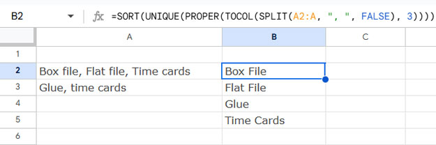
Option 1: Changing Case Before Extraction

=SORT(UNIQUE(PROPER(TOCOL(SPLIT(A2:A, ", ", FALSE), 3))))

This formula extracts unique items while formatting the output to proper case.
If needed, replace PROPER with LOWER or UPPER to format the results accordingly.

Option 2: Keeping the Original Case

If you don’t want to modify the case but still want case-insensitive uniqueness, use:

=LET(list, A2:A, uniqueL, SORT(TOCOL(SPLIT(list, ", ", FALSE), 3)), FILTER(uniqueL, COUNTIFS(uniqueL, uniqueL, SEQUENCE(ROWS(uniqueL)), "<="&SEQUENCE(ROWS(uniqueL))) = 1))

If “Apple” and “apple” both appear, this method retains the first occurrence while ignoring case differences.

Extracting Unique Values from a Comma-Separated List – Case-Sensitive

Assume you have item codes stored in A2:A. To extract unique values while preserving case differences, use:

=SORT(UNIQUE(TOCOL(SPLIT(A2:A, ", ", FALSE), 3)))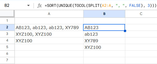

Extracting Unique Values from a Comma-Separated List – Case-Sensitive

How It Works:

SPLIT separates the comma-separated values into individual cells.
TOCOL arranges them into a single column.
UNIQUE removes duplicates while maintaining case sensitivity.
SORT orders the values alphabetically and ensures SPLIT works correctly in an array formula.

Extracting Unique Values from a Comma-Separated List – Case-Insensitive

If you want to ignore case differences while extracting unique values, follow these methods.

Solution 1: Changing Case

=SORT(UNIQUE(PROPER(TOCOL(SPLIT(A2:A, ", ", FALSE), 3))))

This method ensures that similar values like apple and Apple are treated as the same and formatted accordingly.
Replace PROPER with LOWER or UPPER if you prefer a different text format.

Extracting Unique Values from a Comma-Separated List – Case-Insensitive with Case Formatting

Solution 2: Without Changing Case

If you want case insensitivity but prefer to retain the original text format, use:

=LET(list, A2:A, uniqueL, SORT(TOCOL(SPLIT(list, ", ", FALSE), 3)), FILTER(uniqueL, COUNTIFS(uniqueL, uniqueL, SEQUENCE(ROWS(uniqueL)), "<="&SEQUENCE(ROWS(uniqueL))) = 1))

This method ensures that the first occurrence of a value is kept in its original case while removing duplicates case-insensitively.

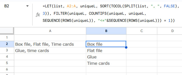
Extracting Unique Values from a Comma-Separated List – Case-Insensitive without Case Formatting

Explanation:

SORT(TOCOL(SPLIT(list, ", ", FALSE), 3)) – Splits the list, arranges items into a column, and sorts them.
FILTER(uniqueL, COUNTIFS(uniqueL, uniqueL, SEQUENCE(ROWS(uniqueL)), "<="&SEQUENCE(ROWS(uniqueL))) = 1) – Filters unique values without altering their original format.

Conclusion

We explored three different ways to extract unique values from a comma-separated list in Google Sheets:

Case-Sensitive Extraction – Useful for passwords, item codes, or any data where case matters.
Case-Insensitive Extraction (Changing Case) – Suitable for names, product names, or other text where formatting is acceptable.
Case-Insensitive Extraction (Preserving Case) – Ideal when you want unique values while maintaining their original format.

For more advanced methods, you can check out these related guides:

9 COMMENTS

S March 24, 2022 At 10:42 pm

Can this be done in the Excel online workbooks?

- Prashanth March 25, 2022 At 7:05 am
  
  Hi, S,
  
  We can do it. But remember, at present, SPLIT() is not available in Excel.
  
  There is a workaround formula.
  
  For formula explanation, please check this guide. In that, you can find a step#4 formula.
  
  Wrap that formula output with UNIQUE, then SORT.
  
Zaim May 7, 2021 At 8:58 am

Hi Prashanth.

Please help how to have an ArrayFormula only in B2 (so B3 and B4 will get the value from the formula in B2).

List of Items
A2: Box File, Flat File, Time Cards, Box File
A3: Glue, Time Cards, Glue, Glue
A4: Pencil, Pen, Glue, Pen

Extracted Unique List (Expected result)
B2: Box File, Flat File, Time Cards
B3: Glue, Time Cards
B4: Pencil, Pen, Glue

Thank you in advance.

- Prashanth May 7, 2021 At 11:13 am
  
  Hi, Zaim,
  
  I suggest a drag-drop formula in B2.
  
  =ArrayFormula(textjoin(", ",true,unique(trim(split(A2,",")),true)))
  
  Since you want an array formula, try the below one.
  
  =ArrayFormula(TRIM(transpose(split(textjoin(", ",true, if(row(indirect("A2:A"&counta(left(filter(iferror(unique(flatten( TRIM(split(substitute(if(len(A2:A99),row(A2:A99)&" "&A2:A99,),",", ", "&row(A2:A99)),","))))),iferror(unique(flatten(TRIM(split( substitute(if(len(A2:A99),row(A2:A99)&" "&A2:A99,),",",", "& row(A2:A99)),",")))))<>""),1))+1))-match(left(filter(iferror( unique(flatten(TRIM(split(substitute(if(len(A2:A99),row(A2:A99)& " "&A2:A99,),",",", "&row(A2:A99)),","))))),iferror(unique( flatten(TRIM(split(substitute(if(len(A2:A99),row(A2:A99)&" "&A2:A99,), ",",", "&row(A2:A99)),",")))))<>""),2),left(filter(iferror(unique( flatten(TRIM(split(substitute(if(len(A2:A99),row(A2:A99)&" "&A2:A99,),",",", "&row(A2:A99)),","))))),iferror(unique(flatten(TRIM(split(substitute(if( len(A2:A99),row(A2:A99)&" "&A2:A99,),",",", "&row(A2:A99)),",")))))<>""),2),0)=1,"|",)&ArrayFormula(mid(filter(iferror(unique(flatten(TRIM( split(substitute(if(len(A2:A99),row(A2:A99)&" "&A2:A99,),",",", "& row(A2:A99)),","))))),iferror(unique(flatten(TRIM(split(substitute(if( len(A2:A99),row(A2:A99)&" "&A2:A99,),",",", "&row(A2:A99)),",")))))<>""), 3,150))),"|"))))
  
  Note:
  
  1. Set to work from row 2 to 99.
  2. After each comma separating the words, there should be a white space as shown in your example.
  
  - Zaim May 7, 2021 At 1:36 pm
    
    Wow, the ArrayFormula, the length… But amazing solution.
    Let me test it in my real data first.
    Thanks again. You’re great.
    
    - Prashanth May 15, 2021 At 3:55 pm
      
      Hi, Zaim,
      
      I have a polished version of the formula for an open range. Please visit the below page for the tutorial and sample sheet.
      
      Remove Duplicates from Comma-Delimited Strings in Google Sheets.
      
Atiq August 13, 2020 At 4:47 pm

Need help. How will I be able to count unique numbers separated by commas in one cell?

eg: 1234,2345,6543,3456,1234

Here I have 5 transaction numbers out of which I have 1 duplicate. How can I use the formula to calculate only the unique count of transactions in the cell?

P.S. I am using Google Sheets.

- Prashanth August 15, 2020 At 9:32 am
  
  Hi, Atiq,
  
  Assume the above comma-separated list of numbers is in cell A1. Here is the formula to use and the formula explanation.
  
  =count(unique(TRANSPOSE(split(A1,","))))
  
  Split – split the numbers to individual cells (in columns)
  Transpose – to change the orientation (numbers in columns to rows) so that we can apply Unique.
  Unique – to remove duplicates
  Count – to count the unique values (use Counta if the values are text)
  
J Beazley May 15, 2019 At 3:33 pm

Here is my more concise answer to the same problem:

=UNIQUE(SORT(TRANSPOSE(SPLIT(JOIN(", ", E2:E), ", ", FALSE))))

For other visitors, note that TRANSPOSE needs to go around the SPLIT, otherwise your SORT/UNIQUE operations will not work.