When preparing quarterly summary reports, you might want to extract the quarter from a date in Google Sheets automatically.

In this post, we’ll explore how to extract the quarter from a date, as well as the quarter with the year. If you want to apply this to a range of dates, the best option is using the QUERY function, which has a scalar function called QUARTER. Let’s dive into the examples below.

The Proper Way to Extract Quarter from a Date in Google Sheets

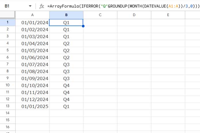
Assume the date is in cell A1. To extract the quarter in the format “Qn” (e.g., “Q1”), you can use the following formula in cell B1 (or any empty cell):

=IFERROR("Q"&ROUNDUP(MONTH(DATEVALUE(A1))/3,0))

• You can replace "Q" with "Quarter" or remove "Q"& if you prefer the quarter in numeric format.
• The formula returns an empty cell if A1 contains text (not a date formatted as text), non-date numeric values, or is empty.

The DATEVALUE function ensures the MONTH function correctly interprets the input as a date. Without DATEVALUE, if A1 is empty, MONTH would incorrectly return 12 (since empty cells are treated as 0, which corresponds to 30/12/1899), or it may return other incorrect results for numeric inputs.

The IFERROR function prevents errors from invalid inputs, leaving the cell empty instead.

Apply the Formula to a Range of Dates

To apply this formula to the range A1:A, you can either drag the formula down or convert it to an array formula:

=ArrayFormula(IFERROR("Q"&ROUNDUP(MONTH(DATEVALUE(A1:A))/3,0)))

• Replace A1:A with the desired date range.
• Before entering the formula, ensure cells B1:B are empty for the array formula to work properly.

Extract Quarter and Year from a Date in Google Sheets

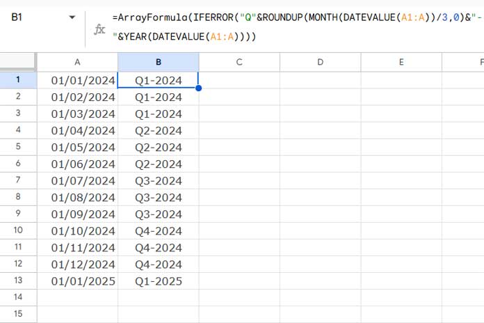
To extract both the quarter and the year from a date, use this formula:

=IFERROR("Q"&ROUNDUP(MONTH(DATEVALUE(A1))/3,0)&"-"&YEAR(DATEVALUE(A1)))

This returns the result in the format "Qn-year" (e.g., Q1-2024).

• Replace "Q" with "Quarter" if you prefer.
• Like before, DATEVALUE and IFERROR ensure the formula handles only valid date inputs.

Array Formula Version:

=ArrayFormula(IFERROR("Q"&ROUNDUP(MONTH(DATEVALUE(A1:A))/3,0)&"-"&YEAR(DATEVALUE(A1:A))))

This applies the formula to the entire column A.

Using the QUARTER Scalar Function in QUERY

If you want to extract the quarter in numeric format from a date range, the QUERY function provides a straightforward option. You can also extract the year into a second column.

For the date range A1:A, use this formula to extract the quarter:

=QUERY(A1:A, "SELECT QUARTER(Col1) LABEL QUARTER(Col1)''", 0)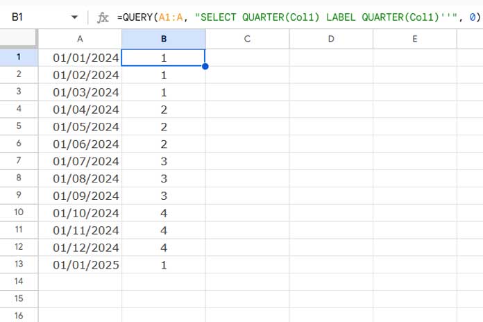

To extract both the quarter and the year into two columns:

=QUERY(A1:A, "SELECT QUARTER(Col1), YEAR(Col1) LABEL QUARTER(Col1)'', YEAR(Col1)''", 0)

This avoids complex calculations by leveraging the scalar functions.

Resources

• Group Dates in Pivot Table in Google Sheets (Month, Quarter, and Year)
• Formula to Group Dates by Quarter in Google Sheets
• Query to Create Daily/Weekly/Monthly/Quarterly/Yearly Report Summary in Google Sheets
• Query Quarter Function in Non-Calendar Fiscal Year Data (Google Sheets)
• Convert Dates to Fiscal Quarters in Google Sheets
• Current Quarter and Previous Quarter Calculation in Google Sheets
• How to Calculate Average by Quarter in Google Sheets
• Sum By Quarter in Excel: New and Efficient Techniques