")
")


")


")

")
")
 in Excel & Google Sheets")


Sometimes, you might want to look at your data from different angles—maybe sorted by product this time, by region the next, or by volume after that. If you’re using the SORT function manually, that means editing the formula every time. Not fun.
But there’s a better way.
You can dynamically sort by column and order in Google Sheets. With this setup, you just pick the field name and sort order from dropdowns, and the formula updates automatically. No need to touch the formula again.
You can sort by just one column or multiple columns. And if you don’t pick anything, it simply shows the data as-is—unsorted.
Let’s walk through how it works.
Sample Data
Here’s some sample data we’ll use to build our dynamic sort formula:
| Product | Region | Volume | Revenue (USD) |
|---|---|---|---|
| Safety Goggles | West | 320 | 6,400 |
| Fire Extinguisher | East | 45 | 6,750 |
| Gloves | North | 1,200 | 3,600 |
| Smoke Detector | South | 80 | 4,800 |
| Safety Goggles | East | 250 | 5,000 |
| Fire Extinguisher | West | 38 | 5,700 |
| Gloves | South | 1,050 | 3,150 |
| Smoke Detector | North | 95 | 5,700 |
Enter this data in the range A1:D.
We’ll set things up so you can sort this data dynamically by Product, Region, Volume, or Revenue, in either ascending or descending order.
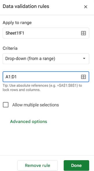
Step 1: Create Dropdowns for Sort Columns
- Click on cell F1.
- Go to Insert > Dropdown.
- Under “Criteria,” choose Dropdown (from a range).
- Set the range to
A1:D1(your header row), then click Done.
Copy and paste the dropdown into F2:F4 if you want to allow multiple levels of sorting.
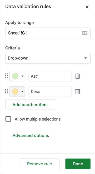
Step 2: Create Dropdowns for Sort Order
- In cell G1, go to Insert > Dropdown.
- Replace Option 1 with
Ascand Option 2 withDesc.
Copy and paste this dropdown into G2:G4 to match the number of columns you might want to sort.
You don’t have to use all the dropdowns. But having more gives you flexibility for multi-column sorting when needed.
Step 3: Add the Formula
Now for the magic.
Once you’ve picked your sort columns and sort orders in columns F and G, the following formula will sort your data based on your selections.
Here’s the formula:
=LET(
   data, A1:D, drop_down, F1:G4, df, SORTN(drop_down, 9^9, 2, 1, TRUE),
   IFERROR(
      QUERY(
         FILTER(data, LEN(TRIM(TRANSPOSE(QUERY(TRANSPOSE(data),,9^9))))),
         "select * order by "&
         TEXTJOIN(", ", TRUE, INDEX(IFNA("Col"&XMATCH(CHOOSECOLS(df, 1), CHOOSEROWS(data, 1))&" "&CHOOSECOLS(df, 2))))
      ),
      {data}
   )
)
How the Formula Works (in Simple Terms)
datais your full dataset (A1:D).drop_downis your drop-down range (F1:G4), where:- F1:F4 contains the columns you want to sort by (e.g., Region, Volume).
- G1:G4 contains the sort order (Asc or Desc).
dfuses SORTN to remove duplicate fields selected in the drop-down.XMATCHfinds the correct column number for each header.TEXTJOINcreates a dynamic string likeCol2 asc, Col1 desc, which the QUERY function uses to sort.FILTER(...TRANSPOSE...)removes truly blank rows so they don’t get pulled to the top of the sorted results.- If there is an error (for example, an empty field/column selection in the drop-down), IFERROR returns the original unsorted data.
Tips for Using Dynamic Sort
- You don’t need to select all dropdowns. Just pick the columns and sort orders you need.
- If nothing is selected, the formula returns the original unsorted data.
- New: If you select the same field (column) multiple times in the drop-down, the formula automatically removes the duplicate selection.
- If the sort order in column G is blank or set to “Asc,” the formula automatically sorts in ascending order. No need to fill every cell.
- Want more sorting levels? Just extend the dropdowns in columns F and G.
Why This Method Is Useful
- No need to rewrite formulas.
- You can change the sort column and order on the fly.
- It works great for dashboards and interactive reports.
- Supports multiple levels of sorting (like Region first, then Product).
Conclusion
This method makes it easy to dynamically sort data by column and order in Google Sheets without touching the formula again and again. It’s simple to set up, flexible to use, and works great for any dataset where you want full control over how it’s sorted.
Related Tutorials
- Sort by Custom Order in Google Sheets
- Sort by Month Name in Google Sheets
- Sort by Field Name Instead of Column Letter in Google Sheets
- How to Sort by Date of Birth in Google Sheets
- Sort Items by Number of Occurrences in Google Sheets
- Sort by Day of the Week in Google Sheets
- Sort by Partial Match in Google Sheets
- Sort Data with Line Breaks in Cells
- Keep Blank Rows While Sorting in Google Sheets
- Sort Column by Text Length in Google Sheets
Prashanth,
Thank you very much for posting this handy tutorial.
In my adaptation, the sorting did not work if any of the sort-by dropdowns contained the same selection (perhaps left over from a previous sort). After spending a few hours working through the LET command, I concluded that this issue occurs because the QUERY function does not allow the same sort column to appear more than once. Please consider enhancing your tutorial by either mentioning this limitation or improving the code to prevent the same column from being passed to the QUERY function more than once.
Thank you again for your tutorial.
Thanks for your valuable suggestion! I’ve updated the formula to handle duplicate column selections. Really appreciate your input.
Hi!
I can not get it to work.
The function is not working together with MATCH. It’s not connecting the strings. Any ideas?
Hi, Sandra,
Please check your Sheets’ LOCALE settings under the FILE menu.