Here is a simple trick you can use to get a dynamic index column in VLOOKUP. You can follow two methods in Google Sheets to achieve this. What are they?
- Create a virtual array (VLOOKUP range) and freeze the index column number. In this case, the index column number remains constant. For example, the index column number might always be 2, even if you delete or insert new columns. This brings dynamism to the index column while keeping the same reference.
- Use the COLUMN function as the index number. This automatically adjusts the VLOOKUP index column when you delete or add new columns in the range.
Suppose you have a 5-column dataset, and you want to return a value from column 3 based on a lookup in column A. In this case, column 3 is your index column.
Now, what happens when you insert a new column between columns 1 and 2, or between columns 2 and 3? The index column number in your VLOOKUP will still be 3, but it should now be 4 because the column positions have shifted.
You can “freeze” the third column (not the index number itself) in VLOOKUP, regardless of its position or index number. Let me explain this concept, called a dynamic index column in VLOOKUP, in Google Sheets.
Tips to Get a Dynamic Index Column in VLOOKUP in Google Sheets
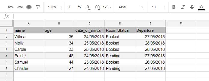
Sample Data:

In this example, I want to look up a name in column A to retrieve that person’s date_of_arrival, which is in column C.
In VLOOKUP, the index number for the date_of_arrival column is 3. How can we freeze this index column (not the column number) in Google Sheets?
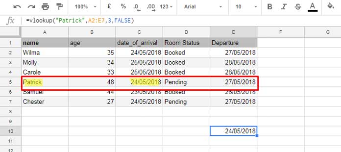
First, let’s see a standard VLOOKUP formula that returns the date_of_arrival based on the lookup name “Patrick”:
=VLOOKUP("Patrick", A2:E7, 3, FALSE)
This formula looks for the name “Patrick” in column A, within the range A2:E7, and returns the value from column 3 (the date_of_arrival) in the corresponding row.
In this formula, the column index is not dynamic. This means if you insert a new column after columns A or B, the index number should now be 4, since the date_of_arrival column has shifted to position 4. However, in the formula, it will still reference 3.
As mentioned earlier, you can freeze the index column (not the column number) in two ways in Google Sheets.
Dynamic Index Column Formulas
Formula 1: Get Dynamic Index Column in VLOOKUP in Google Sheets
=VLOOKUP("Patrick", A2:G7, COLUMNS(A2:C7), FALSE)Formula 2: Get Dynamic Index Column in VLOOKUP in Google Sheets
=VLOOKUP("Patrick", {A2:A7, C2:E7}, 2, FALSE)The first formula makes the index number dynamic by using the COLUMNS function. The COLUMNS function counts the columns from A to C and returns the number 3. This number is then used as the column index in the VLOOKUP formula.
When you insert or add new columns between columns A and C, the column index number will change dynamically.
The second formula follows a different approach to create a dynamic index column in VLOOKUP.
In this formula, the column index number remains 2, regardless of the actual column index. This is because the lookup range only includes the first column (the lookup column), followed by the range starting from the index column.
For example, our original data range is A2:E7, but in VLOOKUP, I modified this range to {A2:A7, C2:E7}, effectively skipping the columns between columns A and C.
This way, any changes such as inserting or deleting new columns won’t affect the formula.
Conclusion
The two methods above are the easiest ways to make the index column dynamic in VLOOKUP in Google Sheets.
Of course, you can also use INDEX-MATCH as an alternative, but VLOOKUP remains the simplest and most straightforward option.


