")
")


")


")

")
")
 in Excel & Google Sheets")


The DATEVALUE function in Google Sheets is designed to convert a date string into a serial date value. However, it also serves two other key purposes:
- Replacing the ISDATE drag-down formula or the alternative MAP + ISDATE combination.
- Simplifying the use of date conditions in the QUERY function.
A date value in Google Sheets is a number representing the number of days since December 30, 1899. For example, the DATEVALUE function returns 1 for the date string “1899-12-31” and 2 for “1900-01-01”.
Syntax of the DATEVALUE Function
The syntax of the DATEVALUE function in Google Sheets is:
DATEVALUE(date_string)Where date_string is a text string that represents a date. If you hardcode the date string, it must be enclosed in double-quotes.
Example:
=DATEVALUE("05/09/23")The date_string can be in any format that Google Sheets recognizes. Here are some examples of valid date string formats:
05/09/23Tue, 05 09 23Tue, 5 Sep 20232023-09-055 Sep 20235-Sep-202305/09Tuesday, 5 September 2023Tuesday, 5 September 2023, 10:10:3013:25(time only)
When interpreting a date string, Google Sheets uses the Locale setting, determining whether the format is MM/DD/YYYY or DD/MM/YYYY. For instance, the date string “05/09/2023” may be interpreted as May 9, 2023, or September 5, 2023, depending on your Locale. You can check your locale’s date formatting by entering the =TODAY() function in a new sheet.
Exception: If the date string contains a month in text format, like “5 Sep 2023”, there won’t be an issue with different date formats.
Examples
In the following example, I’ve used the DATEVALUE function to convert date strings in the range A3:A11 into date values:
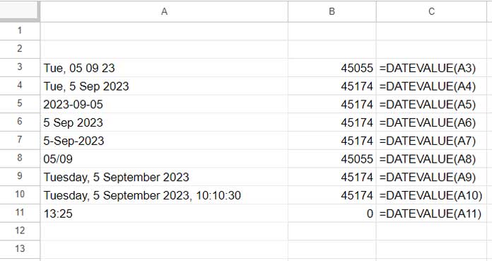
To convert a single date string (cell A3) to a date value, use:
=DATEVALUE(A3)To apply the formula to a range of cells at once, use the following array formula in B3:
=ARRAYFORMULA(DATEVALUE(A3:A11))This converts all date strings in the range A3:A11.
How to Convert DATEVALUE to Date Format in Google Sheets
There are two ways to convert a serial number back to a readable date format:
- Using the TO_DATE Function
The TO_DATE function converts a date serial number into a date.
Syntax:
TO_DATE(value)For example, to convert the serial number returned by the DATEVALUE function back to a date:
=TO_DATE(DATEVALUE("Tue, 5 Sep 2023"))When converting a range of serial numbers, wrap the TO_DATE function in ARRAYFORMULA:
=ARRAYFORMULA(TO_DATE(DATEVALUE(A3:A11)))- Using Number Formatting
Alternatively, you can format the serial number using Format > Number > Date in the menu.
Other Uses of the DATEVALUE Function
- Replacing ISDATE and MAP with DATEVALUE
The ISDATE function checks if a cell contains a valid date, time, or timestamp and returns TRUE or FALSE.
Syntax:
ISDATE(value)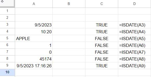
If you want to apply ISDATE to a range of cells, you typically combine it with the MAP function:
=MAP(A3:A9, LAMBDA(r, ISDATE(r)))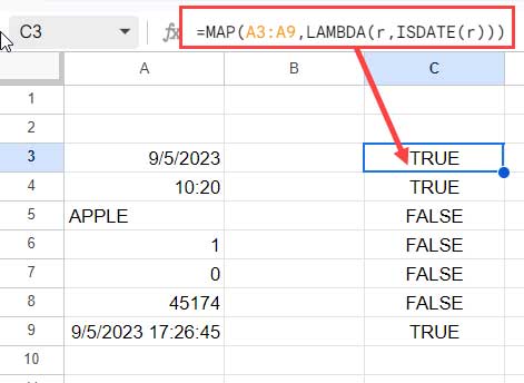
Alternatively, the DATEVALUE function can be used to achieve this and distinguish between dates and times.
=ARRAYFORMULA(IFERROR(DATEVALUE(A3:A9), -1) >= 0)This formula returns TRUE for valid dates and FALSE for invalid date strings or times.
If you need to return FALSE for cells containing only time (without a date), use:
=ARRAYFORMULA(IFERROR(DATEVALUE(A3:A9), -1) > 0)Key Difference: The ISDATE function will return TRUE if the cell contains a number formatted as a date (e.g., formatted as ‘Sunday’). In contrast, DATEVALUE will return an error if the text cannot be converted to a date.
- Simplifying Date Conditions in QUERY with DATEVALUE
Handling date literals in the QUERY function can be tricky. Using the DATEVALUE function simplifies this process.
Assume you have an expense sheet with dates in column A, expense types in column B, and beneficiary names in column C. To filter the data between two dates in cells E2 and E3, you would typically use a QUERY formula like:
=QUERY({A2:C}, "Select * where Col1 > date '"&TEXT(E2,"yyyy-mm-dd")&"' and Col1 < date '"&TEXT(E3,"yyyy-mm-dd")&"' ")However, using DATEVALUE, you can simplify the formula:
=ARRAYFORMULA(QUERY(HSTACK(DATEVALUE(A2:A), B2:C), "Select * where Col1 > "&E2&" and Col1 < "&E3&" "))This method allows the use of number literals for date comparisons. Alternatively, you can apply Format > Number > Number to column A and use:
=QUERY(A2:C, "Select * where Col1 > "&E2&" and Col1 < "&E3&"")Conclusion
The DATEVALUE function in Google Sheets is a versatile tool for converting date strings into serial date values. We’ve seen its core uses, along with tips to replace the ISDATE function and simplify date queries.
One final tip: many Google Sheets functions, like SEQUENCE, can automatically generate date values. For example, the following formula returns 31 date values starting from January 1, 2023:
=SEQUENCE(31, 1, "2023-1-1")You can use the TO_DATE function to convert these serial numbers back into proper dates:
=ARRAYFORMULA(TO_DATE(SEQUENCE(31, 1, "2023-1-1")))In summary, while other functions return date values, DATEVALUE is the go-to for converting date strings into date values.