DateTime and Timestamp are two keywords you can use to handle a timestamp column with the QUERY function in Google Sheets. In this tutorial, we’ll discuss how to use these keywords effectively.

Understanding this is essential because you may encounter a timestamp column in Google Forms responses and want to filter or group records based on that column. Additionally, you may record timestamps using Google Apps Scripts or a custom lambda function to log the time of an entry in your sheet.

Let’s dive into how to use DateTime in the QUERY function!

How to Use DateTime in the QUERY Where Clause

Before learning how to use DateTime in the QUERY Where clause, you must understand the concept of Literals in the QUERY language.

Literals are values used for comparisons or assignments. For date/time types, there are three keywords: date, timeofday, and datetime (or timestamp).

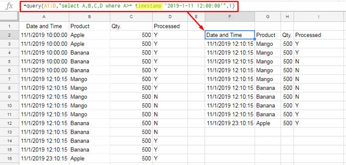
To compare a column containing both date and time, you can use either the datetime or timestamp keyword, as shown below:

Criterion Hardcoded

Formula when column A contains a timestamp/DateTime:

=QUERY(A1:D, "select A,B,C,D where A>= timestamp '2019-01-11 12:00:00'",1)

In the above filter, column A contains the timestamp/DateTime. An alternative Query formula is:

=QUERY(A1:D, "select A,B,C,D where A>= datetime '2019-01-11 12:00:00'",1)

Both formulas will return the same result. Specifically, they retrieve data from columns A to D for rows where the timestamp in column A is greater than or equal to 2019-01-11 12:00:00.

When hardcoding the criterion as shown above, the date must be in the format YYYY-M-D or YYYY-MM-DD, regardless of the date formatting applied to column A.

Criterion as Cell Reference

If you want to use a timestamp from a cell (for example, cell E1) as the criterion, you can modify the formula like this:

=QUERY(A1:D, "select A,B,C,D where A>= datetime '"&TEXT(E1,"yyyy-mm-dd HH:mm:ss")&"' ",1)

You can also replace the datetime keyword with timestamp if needed.

How to Format DateTime in the QUERY Output

When you format a DateTime column using the QUERY format clause, it doesn’t alter the actual DateTime value stored in the cell—it only changes the display format.

This is useful if you want to display the timestamp in a date format while keeping the underlying value intact.

For more details on formatting, see: How to Format Date, Time, and Numbers in Google Sheets QUERY.

The Use of DateTime in the Format Clause:

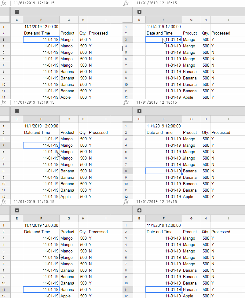
=QUERY(A1:D, "select A,B,C,D where A>= datetime '"&TEXT(F1,"yyyy-mm-dd HH:mm:ss")&"' format A 'DD-MM-YY'",1)

Note that in the formula bar, the value is not in DD-MM-YY format as displayed in column F; it still contains time values. The formatting only masks the time elements, and the underlying value remains unchanged.

You can also format the timestamp to include time:

=QUERY(A1:D, "select A,B,C,D where A>= datetime '"&TEXT(F1,"yyyy-mm-dd HH:mm:ss")&"' format A 'DD-MM-YY HH:MM AM/PM'",1)

Using DateTime in the QUERY Group By Clause

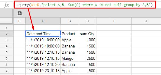
In this example, we’ll group the data based on DateTime in column A and Product in column B:

=QUERY(A1:D,"select A,B, Sum(C) where A is not null group by A,B", 1)

If you examine the result, you’ll see that the DateTime in column F doesn’t show the expected output. This is because it groups by both date and time.

To exclude the time and group only by date, use the toDate scalar function in both the Select and Where clauses as follows:

=QUERY(A1:D, "select todate(A),B, Sum(C) where A is not null group by todate(A),B", 1)

That’s everything you need to know about using DateTime (timestamp) in the QUERY function in Google Sheets. This tutorial covers how to work with a timestamp column effectively.

Resources

• Group and Sum Time Duration Using Google Sheets QUERY
• How to Use Date Criteria in QUERY Function in Google Sheets
• How to Use the DATEDIFF Function in Google Sheets QUERY
• QUERY to Filter Previous N Dates in Google Sheets
• QUERY to Filter Closest Higher Date to Today in Google Sheets
• Month Name as the Criterion in Date Column in QUERY Function in Google Sheets
• How to Add or Subtract N Days to Dates in a Column in Google Sheets QUERY
• How to Use Date Values (Date Serial Numbers) in Google Sheets QUERY