Let’s say we want a formula that returns the cumulative balance against each payment in a column in Google Sheets. In that case, we can use two types of formulas.
- Enter a simple formula in every row in the range.
- A formula in the first row of the range that self expands.
I would prefer the latter one, as it’s more convenient to use.
Whatever your choice, in this Google Sheets tutorial, you will get both the formulas to return cumulative balance against each payment in Google Sheets.
Cumulative Balance against Each Payment – What Does It Mean?
I know I must start this tutorial by answering this question. To explain, Let’s consider the closing balance column in a bank statement.
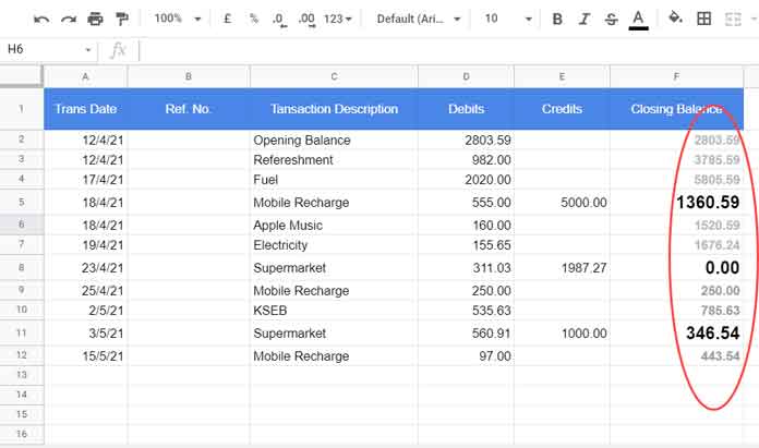
The format of my credit card statement looks like this.

You can see transaction dates, ref. no., description, debits, credits, and closing balance columns. The last column reflects the balance due (cumulative debit including opening balance minus cumulative credit) in each row.
That means Column F contains the cumulative balance. We can use my either of the following running balance formula in cell F2 to populate the values in that column.
Array Formula 1 (for cell F2):
=ArrayFormula(if(len(A2:A),(SUMIF(ROW(D2:D),"<="&ROW(D2:D),D2:D)-SUMIF(ROW(E2:E),"<="&ROW(E2:E),E2:E)),))If you would prefer a simple formula, use the below one in cell F2. It’s a non-array formula. So you should copy this to the rows down.
Non-Array Formula 1:
=sum($D$2:D2)-sum($E$2:E2)I am not going to the detailed formula explanation since I have already covered the same earlier (please follow the link given a few paragraphs above). But I will surely leave some tips at the end part of this tutorial.
Now back to the topic, i.e., cumulative balance against each payment or credit transaction as per the above example.
I want the closing balance only against credits. I want to remove the shaded values (please refer to the image above) in column F. That’s what I meant by the term cumulative balance against each payment in Google Sheets.
I am writing this tutorial as I could see some people prefer to return the cumulative balance against the credits only. Here are the formulas for the same.
How to Return Cumulative Balance against Each Payment in Google Sheets
Non-Array Formula 2:
If we follow the sample data range in the above example, here is the syntax to use.
=if(len(E2),non_array_formula_1,)The expression len(E2) within IF tests whether E2 is blank or not. If blank, it returns a null character, else the cumulative balance up to that row.
In line with the above syntax, here is the formula to use in cell F2.
=if(len(E2),sum($D$2:D2)-sum($E$2:E2),)Drag it down.
Array Formula 2:
Here there is not much changes compared to the above array formula 1.
The LEN in the earlier array formula uses the transaction dates in A2:A to limit the expansion to those rows. Just replace that reference with E2:E (the credit column reference).
The reason for the reference change is we want the cumulative balance against the payments/credits rows only.
So the formula in F2 will be as below.
=ArrayFormula(if(len(E2:E),(SUMIF(ROW(D2:D),"<="&ROW(D2:D),D2:D)-SUMIF(ROW(E2:E),"<="&ROW(E2:E),E2:E)),))The above is the array formula that returns cumulative balance against each payment in Google Sheets.
Formula Explanation
The above is a combination of two SUMIF and one Logical IF formula.
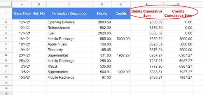
The first SUMIF is an array formula that returns the running total (cumulative sum) of the debits column, whereas the second one returns the cumulative sum of the credit column.
Let’s test them.
In standalone use, you must use =ArrayFormula(if(len(A2:A) with the formulas.
SUMIF 1 (Debits Cumulative Total)
=ArrayFormula(if(len(A2:A),SUMIF(ROW(D2:D),"<="&ROW(D2:D),D2:D),))SUMIF 2 (Credits Cumulative Total)
=ArrayFormula(if(len(A2:A),SUMIF(ROW(E2:E),"<="&ROW(E2:E),E2:E),))In both the SUMIF formulas, only the column (debit/credit) references are different.

SUMIF 1 (debits total) – SUMIF 2 (credits total) is the cumulative balance (please scroll up and see Array Formula 1).
Since we want cumulative balance against payments only, we have replaced A2:A with E2:E. The final formula follows this syntax.
=ArrayFormula(if(len(E2:E),SUMIF_1 - SUMIF_2,))That’s all about how to return cumulative balance against each payment in Google Sheets.
Thanks for the stay. Enjoy!
Resources:


