You can create a weekly summary report in Google Sheets using drag-down formulas, pivot tables, or the QUERY function. We’ll explore each option, starting with basic drag-down formulas.
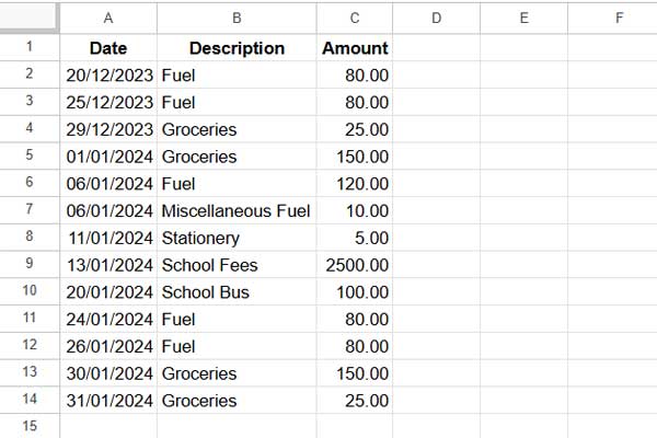
The sample data below contains purchase dates in column A, expense categories in column B, and amounts in column C. Cells A1:C1 contain the field labels “Date,” “Description,” and “Amount.” Let’s create a weekly summary report using this data.
Option 1: Weekly Summary Report Using Helper Columns and Non-Array Formulas
Step 1: Extracting Year and Week Numbers
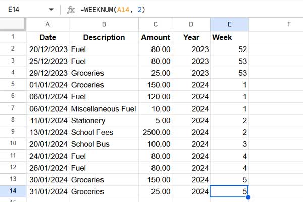
To start, we need to add columns to capture the year and week number of each transaction. First, enter the field labels “Year” in D1 and “Week” in E1.
In cell D2, enter the following formula to get the year, and drag it down:
=YEAR(A2)In cell E2, enter the following formula to get the week number, and drag it down:
=WEEKNUM(A2, 2)This formula calculates the week number based on a Monday-Sunday week (if you want a different start day, replace 2 with the desired number from 1 to 17 as per the WEEKNUM function parameters).
Step 2: Setting Up the Weekly Summary Report Layout
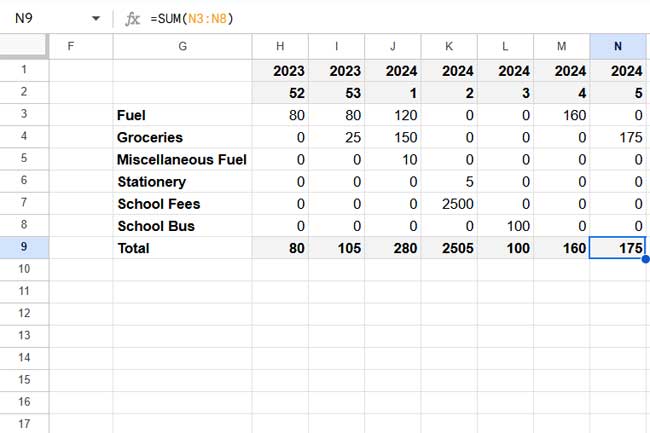
In cell G3, enter the following formula to return unique categories (the TOCOL function removes empty cells):
=TOCOL(UNIQUE(B2:B), 1)In cell H1, enter the following formula to get the unique years and months transposed for the report layout.
=TRANSPOSE(UNIQUE(D2:E))Your weekly summary layout is now ready.
Step 3: Applying the SUMIFS Formula
Use the SUMIFS function to calculate the weekly totals based on the year, week, and category.
In cell H3, enter the following SUMIFS formula and drag it across and down:
=SUMIFS($C$2:$C, $B$2:$B, $G3, $D$2:$D, H$1, $E$2:$E, H$2)You can use the SUM function to add a total below each column in H:N.
Formula Explanation:
- SUMIFS syntax:
SUMIFS(sum_range, criteria_range1, criterion1, [criteria_range2, …], [criterion2, …])- sum_range:
$C$2:$C - criteria_range1:
$B$2:$B - criterion1:
$G3 - criteria_range2:
$D$2:$D - criterion2:
H$1 - criteria_range3:
$E$2:$E - criterion3:
H$2
- sum_range:
Option 2: Weekly Summary Report Using a Pivot Table
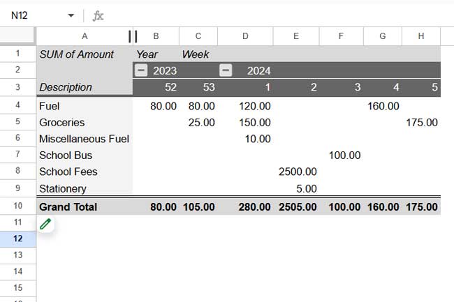
The pivot table option is a quick way to create a weekly summary without complex formulas. Helper columns for year and week (D and E) are required for this method.
Steps:
- Select the range A1:E.
- Go to Insert > Pivot Table > Create, which creates a new sheet for the pivot table layout.
- Drag “Description” to the Rows section.
- Drag “Year” to Columns and then “Week”.
- Drag “Amount” to Values.
- Add Description to Filters and uncheck “Blanks.”
This will provide a pivoted summary by year, week, and category.
Option 3: Weekly Summary Report Using the QUERY Function
Using QUERY is another efficient way to create a weekly summary report. Here, too, we’ll use helper columns for year and week.
=QUERY(A1:E, "SELECT B, SUM(C) WHERE A IS NOT NULL GROUP BY B PIVOT D, E", 1)This formula creates a matrix-style summary, where each row represents a category, and the columns are organized by year and week.
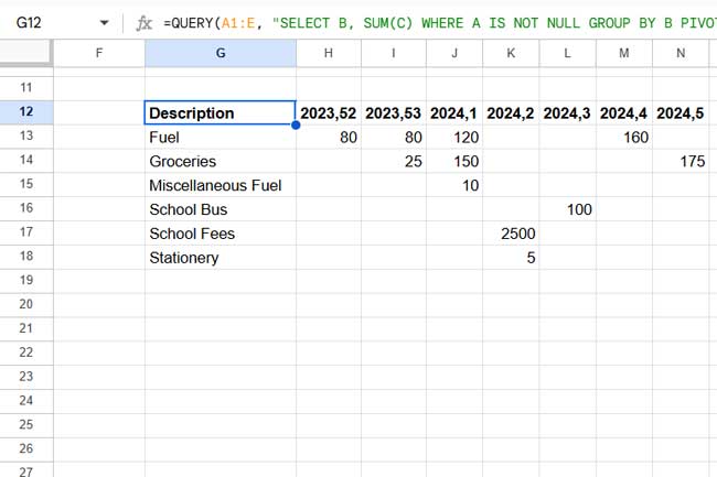
Formula Breakdown:
A1:E: Specifies the range of data to query."SELECT B, SUM(C)": Selects column B (categories) and calculates the sum of values in column C (amounts).WHERE A IS NOT NULL: Ensures only rows with non-empty dates in column A are included.GROUP BY B: Groups the results by each unique category in column B.PIVOT D, E: Creates a pivoted layout, where each combination of values from columns D (Year) and E (Week) becomes a separate column in the output.1: Specifies that the first row contains headers.
This formula provides a summary table that groups expenses by category, year, and week.
Adding a Total Row
To add a dynamic total row, use the following formula and replace your_formula_here with the QUERY formula above:
=ArrayFormula(LET(ftr, your_formula_here, tc, 1, VSTACK(ftr, HSTACK("Total", DSUM(ftr, SEQUENCE(1, COLUMNS(ftr)-tc, tc+1), IFNA(VSTACK(CHOOSEROWS(ftr, 1), )))))))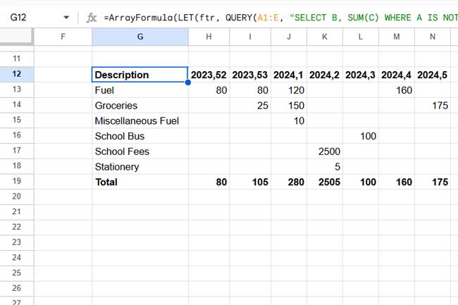
For more information on this approach, check out “Dynamic Total Row for FILTER, QUERY, or ARRAY Results in Sheets.”
Additional Tips
Year Array Formula: Instead of dragging down the year formula, you can use the following array formula in cell D2:
=ArrayFormula(IFERROR(YEAR(DATEVALUE(A2:A))))Week Array Formula: Similarly, replace the week formula with an array formula in E2:
=ArrayFormula(IFERROR(WEEKNUM(DATEVALUE(A2:A), 2)))Resources
- Finding Week Start and End Dates in Google Sheets
- Query to Create Daily/Weekly/Monthly/Quarterly/Yearly Report Summary
- Counting Orders per Week in Google Sheets
- Summarize Data by Week Start and End Dates in Google Sheets
- Dynamic Weekly Averages in Excel Without Helper Columns
This guide provides a comprehensive approach to creating weekly summary reports in Google Sheets using different methods for varying levels of complexity and needs. Choose the approach that best fits your reporting requirements!


In the weekly report, if the result is 0 or null, it is not shown or is ignored. Please help to solve this issue.
Hi, John,
I’m not clear. You can copy my sample sheet and point out the error or leave your suggestions within that sheet.
Share that copy in your comment/reply below.
Hello!
Your formula worked successfully for me!
But I would like to get the Week number to display as the end of week date (Day of Week, Day, Month, Year).
I tried using WEEKDAY formulas but only returned a non-formattable number.
Any suggestions to make this work? Thanks!!
Hi, Lisa,
This may help – Summarize Data by Week Start and End Dates in Google Sheets.
I used the Weeknum formula in this example with mostly success.
It starts at week 2 though. My first date in column A is 1/4/2021, shouldn’t that be Week 1?
Col1is dates andCol10is Price.={query({ArrayFormula(if(len('2021ContractsData'!A2:A),(WEEKNUM('2021ContractsData'!A2:A,2)),)),'2021ContractsData'!A2:J},
"Select Col1, Count(Col10) Where Col2 is not NULL group by Col1 Label Col1 'Week',Count(Col10) 'Contracts'",0)}
I also get an error if I add Sum in the query:
“Error: Unable to parse query string for Function Query Parameter 2: AVG_SUM_ONLY_NUMERIC”
Thank you for the multitude of pages and instructions.
Hi, Gene Wilkins,
I have tested your formula. It has one issue.
We have added one virtual column to the data that contains week numbers. It’s column # 1.
So the Sum and Count must be performed on column 11, not on column 10.
={query({ArrayFormula(if(len('2021ContractsData'!A2:A),(WEEKNUM('2021ContractsData'!A2:A,2)),)),'2021ContractsData'!A2:J},
"Select Col1, Count(Col11), Sum(Col11) Where Col2 is not NULL group by Col1
Label Col1 'Week',Count(Col11) 'Contracts',Sum(Col11) 'Amount'",0)}
Regarding the issue with the week number, please check the functions WEEKNUM and ISOWEEKNUM on my function guide.
I tried applying the formula as is to my data and restructured my data to reflect exactly what is shown in the examples above. I’m getting the following error code.
Error
“Function ARRAY_ROW parameter 2 has mismatched row size. Expected: 9999. Actual: 9997.”
Hi, rex wu,
Thanks for sharing your sheet that enabled me to find the cause of the said error.
I have updated the formula in this tutorial and also in my sample sheet. That will solve your issue.
Hi,
Thanks a lot for creating these amazing tutorials on Google sheet. I’m learning a lot from you.
I hope you can help me create a similar report like this. Instead of the Week number, I would like to create an array to show the exact first date of that Week number (Monday being the first day and Sunday is the last day).
I’m currently, manually adding a formula on my Datasheet to get that date from your previous post too.
I’m sharing the report to you, hope you can take a look at it.
Thanks in advance.
Hi, Allan,
Please ignore the yellow highlighted helper columns in the “Data” tab. I have added a new column (cyan) that returns week start dates.
Find the below formula in cell G1 in your “Data” tab.
={"Week";ArrayFormula(if(len(A2:A),A2:A-WEEKDAY(A2:A,2)+1,))}You can read the formula explanation HERE.
Regarding the summary based on week start dates, there are four formulas in the “Report” tab. The corresponding cells are highlighted in cyan.
Here is your copy of the Sheet – Weekly Start Date Summary – II.
Best,
Wow, that’s really cool. That is what I need in the report that I’m doing.
If I need to create a report based on Campaign Name. I know I can use some formula like SumIFs and SumProduct to do this. Is there an arrayformula to do this?
Thanks so much.
Hi, Allan,
That seems quite easy!
Copy the formula from B7 to B18 (Report tab) and change the column G to C in both the Select and Group clause in Query. Similarly, copy the B9 formula to B20 and make the above same changes.
You can check my above-shared sheet (Sheet shared in my previous reply) for the modified formulas.
Best,
Very nice! This is very close to what I am looking for.
I tried adjusting with similar data but only created errors. Once I added monthly columns the errors came up.
I have included an example sheet, see the “Modified Days of Week” tab. I also wanted to see the amounts for the current Days of the week.
Link: Removed by admin
Can you help with fixing the errors?
Hi, Howard,
Sorry for the delay in replying. The formula you entered is correct and perfectly follows my instructions. The mistake was from my side!
Sorry to say that I failed to foresee one error related to blank cells in the description and amount columns.
Minor tweaking of the formula can sort out the issue.
You just need to replace the code
query(B6:E)toB6:E. It appears twice in the formula. Please give enough rows and columns for this weekly summary formula to expand.Also please check Formula to Sum by Current Week in Google Sheets.