One of the features of Google Sheets is that you can use open ranges starting from any row, such as A2:A, instead of sticking to A:A, which represents the entire column. When your actual data is in A2:B10, you might choose to use A2:B to accommodate future rows. However, dealing with empty rows can complicate certain operations. COUNTIFS with ‘Not Equal To’ is one such scenario. This tutorial explains how to use COUNTIFS with ‘Not Equal To’ in an infinite (open) range in Google Sheets.

As a side note, you can replace COUNTIFS with SUMPRODUCT, or QUERY in such scenarios. We will explore that later in this tutorial.

Sample Data

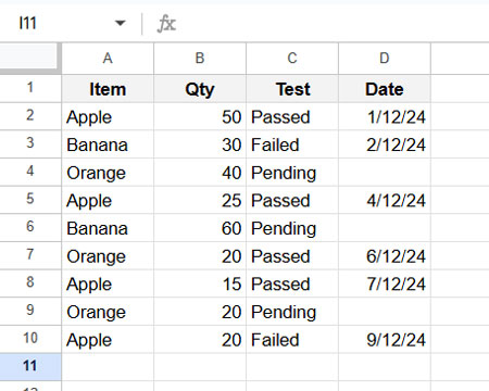
We have the following sample data in A1:D10, which includes Item, Qty, Test, and Date. The Test column represents the quality test status of some fruit items:

The Test column contains statuses such as Pending, Passed, Failed, and blank cells. Sometimes, you may want to count the number of items that are not Passed. Since there are multiple statuses, counting each manually is not ideal.

COUNTIFS with ‘Not Equal To’ in Infinite Ranges

Single Column Example

To count the number of items in the Test column that are not Passed, use the following COUNTIFS formula:

=COUNTIFS(C2:C10, "<>Passed")

This formula returns the count of items that do not have the status Passed. Based on the sample data, this will return 5.

If you use an open range, such as:

=COUNTIFS(C2:C, "<>Passed")

and your sheet has 1000 rows, it will return 995. This includes 990 empty rows plus the count of items that are not Passed, which is 5.

To avoid counting blank cells, modify the formula as follows:

=COUNTIFS(C2:C, "<>Passed", C2:C, "<>")

This formula excludes blank cells and gives the correct result, even for an open range.

Multiple Columns Example

Suppose you want to count the number of items that are not Passed and are not Apple. For a closed range, use:

=COUNTIFS(A2:A10, "<>Apple", C2:C10, "<>Passed")

This formula checks two conditions:

1. The Item column (A) does not equal Apple.
2. The Test column (C) does not equal Passed.

To handle an open range, where empty cells might exist, modify the formula:

=COUNTIFS(A2:A, "<>Apple", C2:C, "<>Passed", A2:A, "<>", C2:C, "<>")

This ensures that blank cells in both columns are excluded.

Note: When specifying "<>Passed", do not leave a space between <> and Passed (e.g., "<> Passed"), as it will result in incorrect calculations.

SUMPRODUCT Alternative to COUNTIFS ‘Not Equal To’

The SUMPRODUCT function is one of the best alternatives to COUNTIFS with ‘Not Equal To’ in fixed or infinite ranges in Google Sheets. In this approach, we evaluate each condition and multiply the results. The sum of the resulting values gives the desired count.

For example:

=ARRAYFORMULA(C2:C<>"Passed")

This formula returns TRUE in rows where the values in column C are not “Passed.”

=ARRAYFORMULA(C2:C<>"")

This formula returns TRUE in rows where the values in column C are not empty.

When you multiply these results, you get 1 wherever both conditions are TRUE, and 0 otherwise. For example:

=ARRAYFORMULA((C2:C<>"Passed")*(C2:C<>""))

If you sum the output, you will get the count of items that are not “Passed” and are not empty:

=SUM(ARRAYFORMULA((C2:C<>"Passed")*(C2:C<>"")))

You can simplify this operation using SUMPRODUCT as follows:

=SUMPRODUCT((C2:C<>"Passed")*(C2:C<>""))

Alternatively:

=SUMPRODUCT((C2:C<>"Passed"), (C2:C<>""))

Adding More Conditions

If you want to count items that are not “Passed” and exclude rows where the Item column (column A) is “Apple,” you can use the following SUMPRODUCT formula:

=SUMPRODUCT((C2:C<>"Passed")*(C2:C<>"")*(A2:A<>"Apple")*(A2:A<>""))

Alternatively:

=SUMPRODUCT((C2:C<>"Passed"), (C2:C<>""), (A2:A<>"Apple"), (A2:A<>""))

QUERY Alternative to COUNTIFS ‘Not Equal To’

The QUERY function automatically excludes blank cells, making it a convenient alternative. However, its SQL-like syntax may seem complex to some users.

To count the number of items that are not Passed, use:

=QUERY(A2:D, "SELECT COUNT(A) WHERE C<>'Passed' LABEL COUNT(A)''")

To count the number of items that are not Passed and not Apple, use:

=QUERY(A2:D, "SELECT COUNT(A) WHERE A<>'Apple' AND C<>'Passed' LABEL COUNT(A)''")

Wrap-Up

In this tutorial, we explored how to use COUNTIFS with ‘Not Equal To’ in both fixed and open ranges, across single and multiple columns. When dealing with complex criteria, it is important to double-check your results using another method. Alternatives include:

• Using SUMPRODUCT
• Employing the QUERY function

By mastering these techniques, you can confidently handle advanced counting scenarios in Google Sheets.

Resources

• How to Use ‘Not Equal To’ in QUERY in Google Sheets
• COUNTIFS with Multiple Criteria in Same Range in Google Sheets
• COUNTIFS in a Time Range in Google Sheets
• Using ‘Not Blank’ as a Condition in COUNTIFS in Google Sheets
• COUNTIF | COUNTIFS Excluding Hidden Rows in Google Sheets
• How To Use COUNTIF or COUNTIFS In Merged Cells In Google Sheets
• Handling Varying Array Sizes in COUNTIFS in Google Sheets
• OR Logic in COUNTIFS Across Multiple Columns in Google Sheets
• COUNTIFS with ISBETWEEN in Google Sheets
• Counting XLOOKUP Results with COUNTIFS in Google Sheets