


")


")

")
")
 in Excel & Google Sheets")


Managing timesheets in Google Sheets can get tricky when punch in (clock in) and punch out (clock out) entries are logged on separate rows. Employers often need both values in the same row to calculate total working hours, print compact reports, or filter employee records efficiently.
In this guide, I’ll show you how to copy punch out times automatically into the punch in row using a custom function (and an alternative formula if you prefer). This solution helps:
- Calculate working hours more easily.
- Eliminate redundant OUT rows when printing or filtering data.
- Keep your timesheet cleaner and more compact.
If you’d rather generate a completely new table with both time in and time out in the same row, check out my previous guide: Combine Time In and Time Out into the Same Row in Google Sheets.
Prerequisites
Before using the PUNCH_IN_OUT_SAME_ROW custom Named Function, make sure your sheet meets these conditions:
- Your data has three columns: Employee ID/Name, Punch Time, and Status.
- The Status column must contain “IN” (clock in) or “OUT” (clock out).
- The table is sorted first by Employee ID/Name and then by Punch Time.
Function Syntax and Arguments
PUNCH_IN_OUT_SAME_ROW(timestamp, id, status)- timestamp → Column containing punch times.
- id → Employee ID (or Name if you don’t use IDs).
- status → Column containing “IN” or “OUT”.
Copy Punch Out Time to the Punch In Row
Here is my sample data:
| Employee ID | Name | Punch Time | Status |
| 15001 | Ben | 01/01/2023 08:30:00 | IN |
| 15001 | Ben | 01/01/2023 18:14:00 | OUT |
| 15001 | Ben | 02/01/2023 08:14:00 | IN |
| 15001 | Ben | 02/01/2023 18:11:00 | OUT |
| … | … | … | … |
In this dataset, to copy Punch Out times to the Punch In rows automatically, you can use one of the following formulas (after importing the function — importing guidance is provided in the next section).
Formula using Employee ID (recommended):
=PUNCH_IN_OUT_SAME_ROW(C2:C, A2:A, D2:D)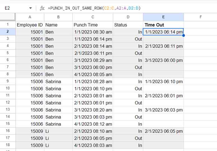
Formula using Name instead of ID:
=PUNCH_IN_OUT_SAME_ROW(C2:C, B2:B, D2:D)After applying either formula, select the output range → go to Format > Number > Date time to display the results properly.
How to Import the Named Function
- Make a copy of my sample sheet.
- Open your own sheet.
- Go to Data > Named functions.
- In the sidebar, click Import function.
- Search for the copied sheet (likely named “copy of clock in_out II”).
- Import the function and confirm.
Now you can use PUNCH_IN_OUT_SAME_ROW just like in the examples above.
Formula Alternative (Without Named Function)
If you don’t want to import a Named Function, you can use the underlying formula directly.
Non-array version (enter in E2 and copy down):
=IF(D2<>"IN",, CHOOSEROWS(IFNA(FILTER(C2:C, A2:A=A2, D2:D="OUT", ROW(A2:A)>ROW(A2))),1))ArrayFormula version:
=MAP(C2:C, D2:D, A2:A, LAMBDA(ac, bc, cc, IF(bc<>"IN",, CHOOSEROWS(IFNA(FILTER(C2:C, A2:A=cc, D2:D="OUT", ROW(A2:A)>ROW(ac))),1))))Formula Breakdown
IF(D2<>"IN", , … )→ Ensures the formula only runs on rows marked as “IN.” If the status is not IN, the cell is left blank.FILTER(C2:C, A2:A=A2, D2:D="OUT", ROW(A2:A)>ROW(A2))→ Finds all punch out times for the same employee ID that occur after the current punch in row.IFNA(..., )→ Prevents errors if no punch out is found.CHOOSEROWS(...,1)→ From the filtered list of punch outs, selects the first one, which corresponds to the next OUT entry.MAP+LAMBDA(array version) → Automates the row-by-row logic for the entire column, so you don’t need to copy the formula down manually.
FAQs
How do I fix a #REF! error in Google Sheets when using this formula?
Array formulas return #REF! if the output column already contains values. Clear column E before applying the formula.
Can I use the Name column instead of Employee ID?
Yes. If you don’t have IDs, replace the id argument with your Name column. Example:
=PUNCH_IN_OUT_SAME_ROW(C2:C, B2:B, D2:D)Do I need to sort my punch in and punch out data first?
Yes. Sort the table first by Employee ID/Name and then by Punch Time. The formula depends on this order to correctly match IN and OUT rows.