Most of us use calendar templates in Google Sheets, where we enter data below dates, such as events, assignments, deadlines, tasks, and reminders. However, analyzing or filtering such data in a grid layout can be challenging. Converting a Google Sheets calendar into a structured table makes it easier to sort, filter, and analyze the data.

In this tutorial, you’ll learn how to convert a Google Sheets calendar into a structured table using a formula. This method extracts events or other information listed under dates and arranges them in a more manageable tabular format—without manual copying or restructuring.

The formula is adaptive, making it suitable for most calendar templates. Please review the prerequisites to understand the calendar requirements for this formula to extract data correctly.

Prerequisites

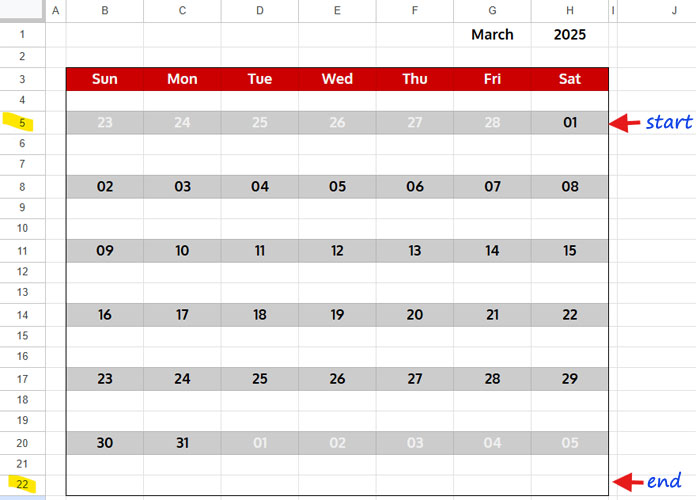
A typical calendar layout in Google Sheets consists of seven columns (for seven days of the week) and six rows (five weeks + one extra row for adjusting weekday padding).

Below each week, you should have additional rows for entering data. The number of rows used for data entry should be consistent for each week. You can use 1 row, 2 rows, 3 rows, etc., depending on your needs, but this structure must remain uniform throughout the calendar.

This is the only prerequisite to convert a Google Sheets calendar into a structured table successfully.

The date row can contain actual dates, dates formatted to display only days, or numbers corresponding to dates. The formula used in this tutorial can effectively identify these rows.

Formula to Convert Google Sheets Calendar into a Structured Table

You can use the following formula to transform a Google Sheets calendar into a structured table:

=LET(
   calendar, B5:H22, 
   row_start, 5, 
   height, 3, 
   seq, SEQUENCE(ROWS(calendar)/height, 1, row_start, height), 
   SORT(REDUCE(TOCOL(,3), SEQUENCE(7), LAMBDA(acc, val, VSTACK(acc, HSTACK(FILTER(CHOOSECOLS(calendar, val), XMATCH(ROW(calendar), seq)), WRAPROWS(FILTER(CHOOSECOLS(calendar, val), NOT(IFNA(XMATCH(ROW(calendar), seq)))), height-1))))))
)

How to Use the Formula

• Replace B5:H22 with your actual calendar range.
• Set row_start to the first row number that contains dates (e.g., 5 in this example).
• Define height as the number of rows allocated per week, including the date row and data entry rows. If you have two rows for data entry below the date row, set height = 3.

The formula will extract and arrange your calendar data into a structured table automatically.

Understanding the Output

If height = 2, the structured table will have two columns:

1. First column: Extracted dates
2. Second column: Corresponding event or data

If height = 3, the structured table will have three columns:

1. First column: Extracted dates
2. Second column: First row of data
3. Third column: Second row of data

Once converted, you can apply filters, lookups, or other data manipulation techniques more efficiently.

Example: Converting a Calendar into a Structured Table

The calendar structure is as follows:

• The range used is B5:H16.
• The range starts at row 5, which contains dates.
• Each week has one row for data entry below the date row, making height = 2.

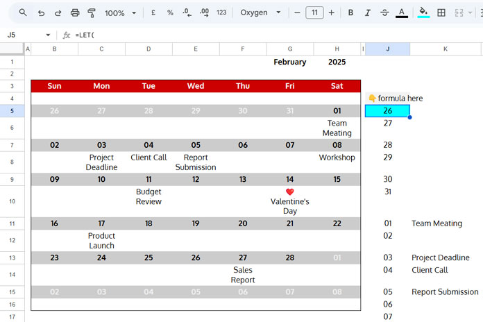
Here is the formula to convert the calendar into a structured table:

=LET(
   calendar, B5:H16, 
   row_start, 5, 
   height, 2, 
   seq, SEQUENCE(ROWS(calendar)/height, 1, row_start, height), 
   SORT(REDUCE(TOCOL(,3), SEQUENCE(7), LAMBDA(acc, val, VSTACK(acc, HSTACK(FILTER(CHOOSECOLS(calendar, val), XMATCH(ROW(calendar), seq)), WRAPROWS(FILTER(CHOOSECOLS(calendar, val), NOT(IFNA(XMATCH(ROW(calendar), seq)))), height-1))))))
)

Since the date row contains actual dates but is formatted to show only days (dd format), the first column in the result also displays days. To view full dates, select the results and go to Format > Number > Date.

Sample Sheet

Formula Explanation

Key Components

1. SEQUENCE(ROWS(calendar)/height, 1, row_start, height)
   • Generates row numbers for date rows (assigned the name seq).
   • Returns a single-column list of row numbers where dates are located.
2. FILTER(CHOOSECOLS(calendar, val), XMATCH(ROW(calendar), seq))
   • Extracts the current column’s dates that match the row numbers in seq.
3. WRAPROWS(FILTER(CHOOSECOLS(calendar, val), NOT(IFNA(XMATCH(ROW(calendar), seq)))), height-1)
   • Filters data rows (excluding date rows) and wraps them into columns based on height.
4. HSTACK(..., ...)
   • Horizontally stacks the extracted date column with its corresponding data.
5. REDUCE + VSTACK
   • Applies this process to each column in the calendar and stacks the results vertically.

This formula efficiently converts a Google Sheets calendar into a structured table while keeping your data intact.

Resources

For further exploration, check out these related tutorials:

• Filter Today’s Events from a Calendar Layout in Google Sheets
• Filter a Custom Made Calendar with Events to a New Sheet in Google Sheets
• Hyperlink Calendar Dates to Events in Google Sheets
• How to Count Events in Particular Time Slots in Google Sheets
• Calendar View in Google Sheets (Custom Template)
• Dynamic Yearly Calendar Template in Google Sheets: Free Template and How-To Guide
• Fully Flexible Fiscal Year Calendar in Google Sheets
• Create Monthly Calendars in Google Sheets (Single & Multi-Cell Formulas)