 in Google Sheets")

")

")


")


")


 mainly in three ways in Google Sheets. They depend on the return value that you are expecting.)
We can compare comma-separated values (CSV) mainly in three ways in Google Sheets. They depend on the return value that you are expecting.
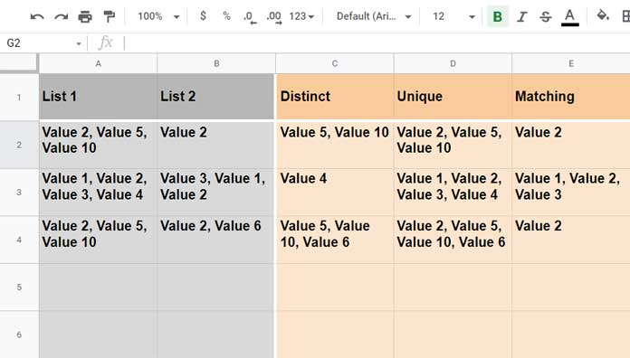
Assume you have CSV set 1 and CSV set 2 as follows in columns 1 and 2.
| CSV Set 1 | CSV Set 2 | Output 1 (DISTINCT) | Output 2 (UNIQUE) | Output 3 (MATCHING) |
| Value 2, Value 5, Value 10 | Value 2 | Value 5, Value 10 | Value 2, Value 5, Value 10 | Value 2 |
I have compared those comma-separated strings/values, i.e., CSV Set 1 and CSV Set2, in three different ways in columns 3 to 5.
Output 1:- It compares CSV 1 with CSV 2 and returns the distinct values.
In this type of comparison, if any value appears in both lists, the formula will omit it in the output.
Output 2:- In this, the formula will remove the duplicates straightaway. So we will get unique values.
Output 3:- In this type of comma-separated value comparison, the formula returns the values that found a match in both CSV sets.
All these serve different purposes in real-life.
Assume someone sent an order to you that contains a long list of books in CSV format.
Later, he has sent a revised order of books in the same format.
Suppose he asks you to send the unique books in both orders or books matching in both. What would you do then?
You can copy those lists into Google Sheets and use my formulas that compare comma-separated values.
Sample CSV Sets and Expected Results
Open a Google Sheets Spreadsheet and enter the values as per the image in cell range A2:B4.
I will provide the formula to insert in C2:E2 (which must be dragged down to C3:E4).
We can use the Unique function to return unique or distinct values in Google Sheets.
So, we will use this function for the first two solutions (columns 3 and 4).
For column 5, we will use Regexmatch since we want to match comma-separated values.
But the above functions won’t work standalone to solve the problem.
Though they are the key, we will use some other functions in the codes to compare the comma-separated values. Here we go!
Compare Comma-Separated Values and Return DISTINCT Values in Google Sheets
We can follow the below syntax in cell C2.
UNIQUE(range,TRUE,TRUE)As I have mentioned earlier, we require some other functions with this UNIQUE function. That’s for the ‘range’ parameter.
We have CSVs to compare in A2 (“Value 2, Value 5, Value 10”) and B2 (“Value 2”).
First, we must combine them using the TEXTJOIN as below.
=textjoin(", ", true,A2:B2)We will get the output – “Value 2, Value 5, Value 10, Value 2.”
There is no way to compare values in a comma-separated list without splitting them in Google Sheets.
We will do that in the next step using the SPLIT function.
=ArrayFormula(trim(split(textjoin(", ", true,A2:B2),",")))The TRIM removes blank spaces, and ARRAYFORMULA is a must since the former function doesn’t work otherwise.
Now we have four values in four cells.
The above is the ‘range’ parameter within the Unique. Please check the provided syntax above.
=unique(ArrayFormula(trim(split(textjoin(", ", true,A2:B2),","))),true,true)The output will be two distinct values. They are “Value 5” and “Value 10”.
Combine them using another Textjoin and that is the C2 formula.
C2 Formula
=textjoin(", ",true,unique(ArrayFormula(trim(split(textjoin(", ", true,A2:B2),","))),true,true))Drag it to C3:C4.
This way, we can compare two comma-separated value sets and return only the distinct values in Google Sheets.
Compare Comma-Separated Values and Return UNIQUE Values in Google Sheets
This time we can use the just above formula with only one correction that is within Unique.
Here is the syntax that we can follow in cell D2.
UNIQUE(range,TRUE,FALSE)This time the last parameter is a FALSE!
So we can use the above formula with one change to compare comma-separated values and return the unique values.
D2 Formula
=textjoin(", ",true,unique(ArrayFormula(trim(split(textjoin(", ", true,A2:B2),","))),true,false))Drag it to D3:D4.
Compare Two CSV Sets and Return MATCHING Values
Here we will depend on REGEXMATCH since we want to match values.
Here we can follow the below syntax to compare two CSVs and return TRUE or FALSE.
REGEXMATCH(text, regular_expression)But what we want is to compare comma-separated values and return the matching values, if any (not TRUE/FALSE values).
So, we should use the following syntax in E2.
FILTER(RANGE, CONDITION1)In this, the ‘CONDITION1’ is the above REGEXMATCH. Let me explain it in a few steps.
1. Split A2 based on comma delimiter and Trim white spaces. We will get “Value 2”, “Value 5”, and “Value 10” in three cells.
=ArrayFormula(trim(split(A2,",")))Output:
| Value 2 | Value 5 | Value 10 |
2. Split B2 and combine the output using a Pipe delimiter to form a regular expression to match.
=ArrayFormula(textjoin("|",true,trim(split(B2,","))))3. Match Step 2 values in step 1 values. We can use the Regexmatch as below.
=ArrayFormula(regexmatch(ArrayFormula(trim(split(A2,","))),ArrayFormula(textjoin("|",true,trim(split(B2,","))))))Output (the ‘CONDITION1’ to use in FILTER):
| TRUE | FALSE | FALSE |
Note:- We can clean the above formula later as the multiple array formulas are not required.
4. Filter table_1 if table_2 is equal to TRUE.
=filter(trim(split(A2,",")),regexmatch(trim(split(A2,",")),textjoin("|",true,trim(split(B2,",")))))Note:- Removed array formulas as they are not required within FILTER.
We have already compared the comma-separated values and returned the matching value.
As earlier, we can combine the returned values.
E2 Formula
=TEXTJOIN(", ",TRUE,filter(trim(split(A2,",")),regexmatch(trim(split(A2,",")),textjoin("|",true,trim(split(B2,","))))))Drag it into E3:E4.
Related Resources
- Extract Unique Values from a Comma Separated List in Google Sheets.
- Remove Duplicates from Comma-Delimited Strings in Google Sheets.
- Replace Multiple Comma Separated Values in Google Sheets.
- How to Count Comma Separated Words in a Cell in Google Sheets.
- Sum, Count, Cumulative Sum Comma Separated Values in Google Sheets.
- Vlookup and Comma-Separated Values – Google Sheets Tips.
- Comma-Separated Values as Criteria in Filter Function in Google Sheets.
- Split Comma-Separated Values in a Multi-Column Table in Google Sheets.
- How to Replace Commas within or outside Brackets in Google Sheets – Regex.