


")


")

")
")
 in Excel & Google Sheets")


You can use the XMATCH or REGEXMATCH functions to match comma-separated criteria within the FILTER function in Google Sheets. Which function you choose depends on whether you need the filter to be case-sensitive.
For instance, if you have sample data in columns B2:C, where column B contains product names and column C contains quantities, and the filtering criteria (e.g., “Product 1, Product 11”) are stored in E2, you can use formulas to filter the data accordingly.
To filter case-insensitively, use the following formula:
=FILTER(C2:C, XMATCH(B2:B, TRIM(SPLIT(E2, ","))))For a case-sensitive filter, you can use the following formula:
=FILTER(C2:C, REGEXMATCH(B2:B, "^"&TEXTJOIN("$|^", TRUE, TRIM(SPLIT(E2, ",")))&"$"))In both formulas, C2:C represents the range of values to filter (the result column), B2:B is the range to apply the criteria, and E2 contains the comma-separated search keys. These formulas return all matches based on the criteria specified. If there are multiple search keys, the formulas will return multiple results.
To consolidate the results into a single cell, you can wrap the formula with TEXTJOIN. For example, to combine the results with a comma and space as the separator, use:
=TEXTJOIN(", ", TRUE, FILTER(C2:C, XMATCH(B2:B, TRIM(SPLIT(E2, ",")))))If the results are numeric and you want to calculate the total instead of combining them into text, wrap the formula with SUM:
=SUM(FILTER(C2:C, XMATCH(B2:B, TRIM(SPLIT(E2, ",")))))These approaches allow you to filter your data based on comma-separated values as criteria in the filter, whether your needs are case-insensitive or case-sensitive.
Comma-Separated Values as Criteria in the FILTER Function – Examples
Consider a sample dataset in columns B2:C, where column B contains product names and column C contains quantities. Cell E2 stores the filtering criteria, such as ‘Product 1, Product 11.’
To filter the range C2:C based on the multiple criteria in E2 and combine the results, you can use the following formula in cell F2:
=TEXTJOIN(", ", TRUE, FILTER(C2:C, XMATCH(B2:B, TRIM(SPLIT(E2, ",")))))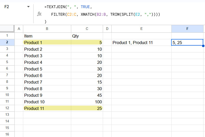
The FILTER function follows this syntax:
FILTER(range, condition1, [condition2, …])Here’s how the components work in this formula:
- range:
C2:C— The range to filter, which contains the values to be returned. - condition1:
XMATCH(B2:B, TRIM(SPLIT(E2, ",")))— The XMATCH function compares the values in B2:B against the split and trimmed values from E2, returning the relative positions of matches or #N/A for non-matches.
The TRIM function removes any extra spaces from the split criteria. The FILTER function then includes rows from C2:C wherever XMATCH finds a match.
This formula performs case-insensitive filtering.
For a case-sensitive alternative, use this formula:
=TEXTJOIN(", ", TRUE, FILTER(C2:C, REGEXMATCH(B2:B, "^"&TEXTJOIN("$|^", TRUE, TRIM(SPLIT(E2, ",")))&"$")))In this case, the condition differs:
REGEXMATCH(B2:B, "^"&TEXTJOIN("$|^", TRUE, TRIM(SPLIT(E2, ",")))&"$")The REGEXMATCH function matches the values in B2:B against the pattern created by:
"^"&TEXTJOIN("$|^", TRUE, TRIM(SPLIT(E2, ",")))&"$"Here’s how the pattern works:
"^"&TEXTJOIN("$|^", TRUE, ...)&"$"creates an OR (|) pattern for all criteria, ensuring that each value is matched exactly.
For example, the pattern ^Product 1$|^Product 11$ matches strings that are exactly “Product 1” or “Product 11.” The FILTER function includes rows from C2:C where the REGEXMATCH condition is TRUE.
Both formulas allow you to filter data based on comma-separated values as criteria in the filter, tailored for either case-insensitive or case-sensitive requirements.
Comma-Separated Values in Multiple Rows as FILTER Criteria
Using the ARRAYFORMULA function with the criteria range E2:E instead of just E2 won’t work here.
To use comma-separated values in multiple rows as the FILTER criterion, you should use the MAP function with a custom lambda function.
The syntax for the MAP function is:
MAP(array1, [array2, …], lambda)Here, array1 is E2:E. For the lambda function, you need to create a custom function using one of the FILTER formulas mentioned earlier.
Case-Insensitive Custom Function:
=LAMBDA(val, TEXTJOIN(", ", TRUE, FILTER(C2:C, XMATCH(B2:B, TRIM(SPLIT(val, ","))))))Case-Sensitive Custom Function:
=LAMBDA(val, TEXTJOIN(", ", TRUE, FILTER(C2:C, REGEXMATCH(B2:B, "^"&TEXTJOIN("$|^", TRUE, TRIM(SPLIT(val, ",")))&"$"))))Once you have the custom function, use it in the MAP function as the lambda. Here’s an example:
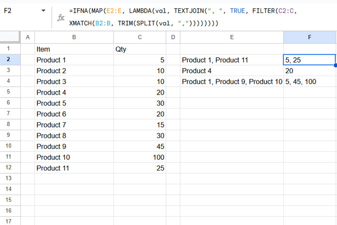
=MAP(E2:E, LAMBDA(val, TEXTJOIN(", ", TRUE, FILTER(C2:C, XMATCH(B2:B, TRIM(SPLIT(val, ",")))))))You should wrap this formula with IFNA to prevent the formula from returning #N/A in empty rows corresponding to E2:E. Here’s how:
=IFNA(MAP(E2:E, LAMBDA(val, TEXTJOIN(", ", TRUE, FILTER(C2:C, XMATCH(B2:B, TRIM(SPLIT(val, ","))))))))This ensures that if a row is empty or contains no matches, the formula will return a blank rather than an error.
Important:
When using these formulas, I suggest sorting the range (B2:C) in ascending order by the first column. Additionally, specify the comma-separated criteria (E2) in the same order.
For example, the criteria should be “Product 1, Product 9, Product 10” rather than “Product 10, Product 1, Product 9.”
While both approaches will return results for all matches, the order of the results will not align with the order of the criteria in the comma-separated list unless the range is sorted properly.