The COLUMNS function returns the number of columns in the specified range, making it a useful component in other functions.

You may find this function in many formulas that use 2D arrays to dynamically calculate the column count and return the desired number of columns.

The syntax of the COLUMNS function in Google Sheets is as follows:

COLUMNS(range)

• range: The array or range whose column count will be returned.

Basic Examples

Before we jump into the examples, it’s important to note that if the number of physical columns is less than the specified range, the formula will return the actual count of physical columns in the range.

For example, the following formulas will return 26 if there are 26 or more columns in your sheet (i.e. if the range extends to or beyond column Z):

=COLUMNS(A1:Z1)
=COLUMNS(A1:Z)

However, if your sheet only contains columns A, B, and C, the formula will return 3, not 26.

Real-Life Uses of the COLUMNS Function

The COLUMNS function in Google Sheets has many practical applications. It helps dynamically select columns in functions such as VLOOKUP, database functions, QUERY, and more. Let’s explore some important use cases.

COLUMNS Function with VLOOKUP

The following VLOOKUP formula searches for “Sophia” in the first column of the range A:G and returns values from columns B to G (2nd to 7th column):

=ArrayFormula(VLOOKUP("Sophia", A:G, {2, 3, 4, 5, 6, 7}, 0))

Instead of manually inputting the index numbers {2, 3, 4, 5, 6, 7}, you can dynamically generate these values using the COLUMNS function with SEQUENCE, as shown below:

=ArrayFormula(VLOOKUP("Sophia", A:G, SEQUENCE(1, COLUMNS(A:G)-1, 2), 0))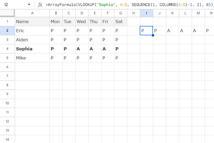

Where:

• =COLUMNS(A:G) will return 7, which is the total number of columns in the range.
• =SEQUENCE(1, COLUMNS(A:G)) will generate the numbers 1 to 7, where 1 is the number of rows and COLUMNS(A:G) is the number of columns.
• To get the column numbers from 2 to 7, you can use:

=SEQUENCE(1, COLUMNS(A:G)-1, 2)

Here, 1 is the row count, COLUMNS(A:G)-1 calculates the number of columns minus the first one, and 2 sets the starting column for the sequence.

COLUMNS Function with Database Functions

There are several database functions in Google Sheets. For example, consider the DGET function:

=ArrayFormula(DGET(A1:G, {2, 3, 4, 5, 6, 7}, {"Name"; "Sophia"}))

The DGET function looks up the name “Sophia” in the “Name” column and returns values from columns 2 to 7.

You can replace the static index numbers {2, 3, 4, 5, 6, 7} with the COLUMNS and SEQUENCE combination as follows:

=ArrayFormula(DGET(A1:G, SEQUENCE(1, COLUMNS(A:G)-1, 2), {"Name"; "Sophia"}))

In this way, the COLUMNS function helps make your formulas more dynamic and adaptable in various real-life scenarios in Google Sheets.

Resources

• Dynamic Column References in Google Sheets QUERY
• Dynamic Formula to Select Every nth Column in QUERY in Google Sheets
• Dynamic Column Id in QUERY IMPORTRANGE Using Named Ranges
• Dynamic Column in VLOOKUP IMPORTRANGE Formula in Google Sheets
• Dynamic Sort Column and Sort Order in Google Sheets