


")


")

")
")
 in Excel & Google Sheets")


In Google Sheets, you might hide rows to declutter large datasets—whether in financial reports, project trackers, or inventory logs. But what if you want to visually highlight the row just above a hidden one?
This can be especially helpful when you want to indicate that something has been hidden below—like completed tasks, irrelevant details, or outliers. Think of a project manager who hides completed rows but wants to flag the last visible task before that collapsed group. In such cases, highlighting the row above each hidden row provides a clear visual cue.
In this tutorial, you’ll learn how to detect hidden rows using a formula and then highlight the row above each one using conditional formatting. It works regardless of how the rows are hidden—manually, by filters, slicers, or groups.
Why Highlight the Row Above a Hidden Row?
There are several practical use cases:
- Project management: Mark the active task just before a batch of hidden (completed) ones.
- Finance dashboards: Signal the end of a month or quarter that’s been collapsed.
- Inventory sheets: Visually separate available stock from archived items.
Whatever the use case, this technique improves clarity without revealing the hidden data.
Important Note Before You Begin
The method described here doesn’t work if there are empty cells in the range where you apply the conditional formatting rule. Make sure the target column (the one used to detect hidden rows) does not contain blank cells within the range where you’re applying the rule.
Step 1: Detect Hidden Rows in Google Sheets (Using Formula)
Google Sheets provides a powerful function to detect visible rows: the SUBTOTAL function.
Enter the following formula to check whether a row is hidden:
=SUBTOTAL(103, A2) = 0How It Works:
SUBTOTAL(103, A2)returns1if the cell in row 2 (column A) is visible.- It returns
0if row 2 is hidden. - So
=SUBTOTAL(103, $A2)=0returnsTRUEwhen row 2 is hidden.
Adjust the formula reference based on your actual range.
For example, if your conditional formatting starts from row 10 in column C, use C11 in the formula instead of A2.
Example:
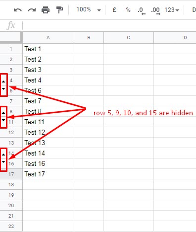
If rows 5, 9, 10, and 15 are hidden, the formula in row 4 (i.e., referencing A5) will return TRUE, and we can use that to highlight row 4.
Step 2: Highlight Row Above Hidden Row in Google Sheets
Now that we can detect a hidden row, let’s apply a conditional formatting rule to highlight the row just above it.
Instructions:
- Select the range where you want to apply the rule — for example,
A1:A100. - Go to Format > Conditional Formatting.
- Under Format rules, select “Custom formula is”.
- Enter this formula:
=SUBTOTAL(103, $A2)=0 - Pick a highlighting color of your choice.
- Click Done.
This formula works because when you’re formatting row 1, it checks whether row 2 is hidden. If it is, row 1 gets highlighted.
Result:
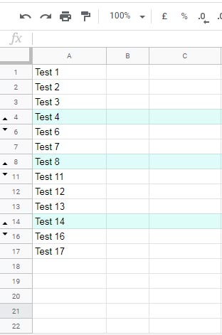
If rows 5, 9, 10, and 15 are hidden, the rule will highlight rows 4, 8, and 14 (the rows immediately above each hidden one).
How to Identify Hidden Rows Manually
While the formula handles detection programmatically, here’s how to spot hidden rows manually:
- Manually hidden rows: You’ll see a small arrow between row numbers.
- Grouped rows: Look for minus (-) or plus (+) signs in the row header. These indicate expandable/collapsible groups.
- Filtered rows: If a filter is applied, hidden rows won’t be numbered consecutively.
These visual indicators can help verify that your formatting rule is working as intended.
Conclusion
This formula-based technique for highlighting the row above each hidden row in Google Sheets is simple yet powerful. Whether you’re using hidden rows for presentation or data cleanup, this formatting trick can improve readability, usability, and workflow visibility.
Just remember:
- The rule doesn’t work with empty hidden cells.
- Always reference the row below in your formula.