The SUMIF function is not case-sensitive in Google Sheets. To perform a case-sensitive SUMIF, you can use the FIND, EXACT, or REGEXMATCH function with the range part of the formula.
For example, to sum the total purchase cost of “apple,” where item names are in column A (A2:A) and costs are in column C (C2:C), you can use either of the formulas below:
- For a partial match:
=ArrayFormula(SUMIF(FIND("apple", $A$2:$A), ">0", $C$2:$C))- For an exact match:
=ArrayFormula(SUMIF(EXACT($A$2:$A, "apple"), TRUE, $C$2:$C))
=ArrayFormula(SUMIF(REGEXMATCH($A$2:$A, "^apple$"), TRUE, $C$2:$C))
Example 1: Case-Sensitive SUMIF Using FIND
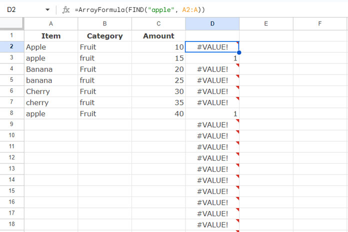
The FIND function returns the position of the first occurrence of a string within a text. In this case, we use “apple” as the string to match cells A2, A3, A4, and so on.
To match the string across multiple cells, we specify the range A2:A and wrap it with the ARRAYFORMULA function.
=ArrayFormula(FIND("apple", $A$2:$A))
This will produce an array of numbers in the matching rows and #VALUE! errors in the non-matching rows. Therefore, we use the FIND formula as the range and “>0” as the criterion. The sum_range will be C2:C.
SUMIF Syntax: SUMIF(range, criterion, [sum_range])
The following formula adheres to the explanation above and returns 55 by case-sensitively matching “apple” in rows 3 and 8.
=ArrayFormula(SUMIF(FIND("apple", $A$2:$A), ">0", $C$2:$C))When using FIND for a case-sensitive SUMIF, consider the potential drawback of partial matches.
For example, it will match not only “apple” but also “apple grade A,” “grade A apple,” etc.
Example 2: Case-Sensitive SUMIF Using EXACT
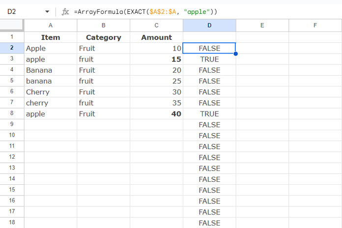
The EXACT function compares two strings and returns TRUE if they are identical, making it case-sensitive.
You can use this function with a range as follows:
=ArrayFormula(EXACT($A$2:$A, "apple"))
This will return an array of TRUE and FALSE values. You can use this array in a SUMIF function for case-sensitive matching. The criterion should be TRUE:
=ArrayFormula(SUMIF(EXACT($A$2:$A, "apple"), TRUE, $C$2:$C))This formula will match the criteria exactly, without partial matches, and is also case-sensitive.
Example 3: Case-Sensitive SUMIF Using REGEXMATCH
If you’re dealing with issues of partial matches, replace the FIND array formula in the range part of SUMIF with the above EXACT formula or the following REGEXMATCH array formula:
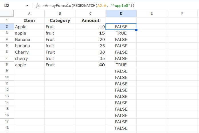
=ArrayFormula(REGEXMATCH($A$2:$A, "^apple$"))
REGEXMATCH is a function for matching regular expressions. This formula matches the regular expression ^apple$ in the range A2:A and returns TRUE for matches and FALSE for non-matches.
It performs a case-sensitive and exact match. In the regular expression, the ^ (caret) asserts the position at the start of a line, and the $ (dollar sign) asserts the position at the end of a line.
The following SUMIF formula uses REGEXMATCH to perform a case-sensitive, exact match of “apple” in A2:A and returns the sum from C2:C:
=ArrayFormula(SUMIF(REGEXMATCH($A$2:$A, "^apple$"), TRUE, $C$2:$C))Advantages of REGEXMATCH Over FIND and EXACT
The FIND function is used for partial matches, while EXACT provides exact matches. However, REGEXMATCH can handle both partial and exact matches.
For partial matches, you can omit the ^ and $ signs in the regular expression.
Additionally, REGEXMATCH makes it easy to specify multiple criteria for case-sensitive SUMIF.
For example, to match multiple strings such as “apple,” “banana,” and “mango,” use the following regular expressions:
- Partial Match:
"apple|banana|mango" - Exact Match:
"^apple$|^banana$|^mango$"
Example:
=ArrayFormula(SUMIF(REGEXMATCH($A$2:$A, "^apple$|^banana$|^mango$"), TRUE, $C$2:$C))Handling Multiple Criteria
Assume you have the criteria “apple” and “banana” in E2 and E3, respectively.
You can use any of the following formulas in F2 and drag it down to F3:
=ArrayFormula(SUMIF(FIND(E2, $A$2:$A), ">0", $C$2:$C))
=ArrayFormula(SUMIF(EXACT($A$2:$A, E2), TRUE, $C$2:$C))
=ArrayFormula(SUMIF(REGEXMATCH($A$2:$A, "^"&E2&"$"), TRUE, $C$2:$C))
In such scenarios, I would suggest using QUERY, which will summarize the data based on the criteria column, case-sensitively:
=QUERY(A:C, "SELECT A, SUM(C) WHERE A<>'' GROUP BY A", 1)Result:
| Item | sum Amount |
| Apple | 10 |
| Banana | 20 |
| Cherry | 30 |
| apple | 55 |
| banana | 25 |
| cherry | 35 |
Resources
- Case Sensitive VLOOKUP in Google Sheets
- How to Perform a Case-Sensitive COUNTIF in Google Sheets
- Case Sensitive Reverse VLOOKUP Using INDEX-MATCH in Google Sheets
- How to Do a Case-Sensitive SUMPRODUCT in Google Sheets
- How to Do a Case-Sensitive DSUM in Google Sheets
- Case-Insensitive REGEXMATCH in Google Sheets (Partial or Whole)
- Case Insensitive UNIQUE in Google Sheets


Hey
Does the QUERY work with the name range (Columns in other tabs)?
Hi, RC,
The Query alternative to case sensitive SUMIF would work with other tabs.
Just include tab name with the Query ‘Data’.
Eg.:
=query('company 1'!A2:G5,"Select Sum(G) where A='IL102b' label Sum(G)''")In this “company 1” is the tab name.