You can calculate a weighted average in a Pivot Table using a custom formula in the calculated field of Google Sheets. While there are a few built-in functions within the Pivot Table, they aren’t suitable for this task because they are specific to individual fields used in the calculation. For a weighted average, you typically need two fields. Therefore, we will rely on the calculated field within the Pivot Table.

We will use the AVERAGE.WEIGHTED function in the calculated field, so there’s no need for any helper columns.

Sample Data

You can enter the following sample data in range A1:D, which represents sales data containing the product, region, price per unit, and units sold:

In this example, we will calculate the weighted average price for each product.

Since we want to calculate the weighted average price of each product, we will use the “Price per Unit” field as the values and the “Units Sold” field as the weights in the AVERAGE.WEIGHTED function. The function syntax is:

AVERAGE.WEIGHTED(values, weights, [additional_values, …], [additional_weights, …])

Steps to Add Weighted Average in the Pivot Table in Google Sheets

It’s quite simple to add a weighted average within a Pivot Table. Here are the steps:

Step 1: Creating the Pivot Table Grid

1. Select the data in range A1:D.
2. Click Insert > Pivot Table.
3. Click Create.

This will create a new sheet with the Pivot Table grid occupying the top-left corner of the sheet.

Step 2: Adding Fields to the Grid

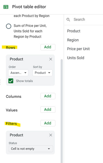
Since we want to group by product, drag and drop the Product field under Rows. Since we are using an open range (A1:D) instead of a fixed range (A1:D7), we should filter out empty rows to avoid errors in the weighted average calculation.

1. Drag and drop the Product field under Filters.
2. Click the filter drop-down (currently set to “Showing all items”) and select Filter by Condition > Cell is not empty.

Step 3: Adding the Weighted Average in the Pivot Table

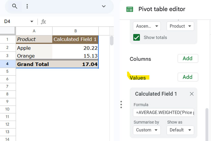
1. Within the Pivot Table editor panel, click the Add button next to Values.
2. Select Calculated Field.
3. In the calculated field, enter the following formula:=AVERAGE.WEIGHTED('Price per Unit', 'Units Sold')
4. Under Summarize by, select Custom.

This will add the weighted average to the Pivot Table.

Formula Explanation

Typically, you would use the following formula to find the weighted average of all items:

=AVERAGE.WEIGHTED(C2:C, D2:D)

When using it within the Pivot Table, you should replace the range references with the corresponding field labels. Field labels must be enclosed in apostrophes.

Since the Pivot Table groups rows by Product, the formula will return the result for each product.

Note: If your field label contains an apostrophe, you should escape it by placing another apostrophe. For example:

• Students’ Scores should be specified as 'Students'' Scores'.
• Student’s Score should be specified as 'Student''s Score'.

Step 4: Customizing the Weighted Average Field Label in the Pivot Table

The above action will leave the field label as “Calculated Field 1” in the first row of the weighted average column in the Pivot Table. You can edit this label by navigating to the cell and updating it in the formula bar to the desired label.

Resources

• Weighted Average of Filtered (Visible) Data in Google Sheets
• Adding Calculated Field in Pivot Table in Google Sheets
• SUMIF in Pivot Table Calculated Fields in Google Sheets
• Weighted Moving Average in Google Sheets (Formula Options)