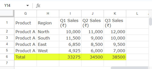
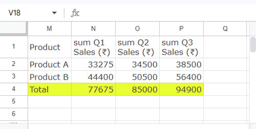
This tutorial explains how to dynamically add a total row to the bottom of array results, such as those generated by FILTER, QUERY, etc., in Google Sheets.
Adding a total row to the bottom of array results like FILTER or QUERY can be challenging, especially when the number of text and numeric columns in the output varies.
We have a dynamic formula that simplifies this process, adjusting automatically when you modify the filter formulas.
Reasons Against Manual Total Rows in Array Results
Manually adding a total row at the bottom can cause errors if the filter formula returns more rows when the source updates.
The FILTER or QUERY function won’t be able to expand due to the manually added total row, resulting in an error. Therefore, users often resort to manually adding the total at the top.
Challenges Adding Total Row Below FILTER or QUERY Results
- There may be multiple columns in the array result for totaling.
- There may or may not be one or more text columns at the beginning of the result.
- The presence of a header row in the result, especially when using QUERY.
We need to manage all these challenges. Our dynamic formula is capable of handling all these issues efficiently.
Sample Data and Filtering
We have sample data structured as Product, Region, Q1 Sales (₹), Q2 Sales (₹), and Q3 Sales (₹) in columns A1:E.
| Product | Region | Q1 Sales (₹) | Q2 Sales (₹) | Q3 Sales (₹) |
| Product A | North | 10,000 | 11,000 | 12,000 |
| Product A | South | 11,500 | 9,000 | 10,000 |
| Product A | East | 6,850 | 8,500 | 9,500 |
| Product A | West | 4,925 | 6,000 | 7,000 |
| Product B | North | 14,900 | 18,000 | 19,875 |
| Product B | South | 12,000 | 14,000 | 15,600 |
| Product B | East | 10,000 | 11,500 | 12,925 |
| Product B | West | 7,500 | 7,000 | 8,000 |
The following FILTER formula filters the table for rows where the Product column matches “Product A”:
=FILTER(A1:E, A1:A="Product A")And the following QUERY formula summarizes the data by grouping products:
=QUERY(A1:E, "SELECT A, SUM(C), SUM(D), SUM(E) WHERE A <>'' GROUP BY A", 1)How do we dynamically place a total row below these outputs?
Adding a Dynamic Total Row Below FILTER, QUERY, or ARRAY Results in Sheets
Before using our dynamic formula, consider whether your formula result includes a header row.
FILTER formula results typically do not include a header row unless explicitly added through stacking or other methods. In contrast, QUERY formula results usually include a header row by default.
The application slightly varies depending on the presence of a header row.
Option 1: Formula Results without Header Row
Here’s the dynamic formula to add a total row below array results that do not have a header row:
=ArrayFormula(LET(ftr, VSTACK(header, your_formula_here), tc, n, VSTACK(ftr, HSTACK("Total", DSUM(ftr, SEQUENCE(1, COLUMNS(ftr)-tc, tc+1), IFNA(VSTACK(CHOOSEROWS(ftr, 1), )))))))Explanation:
- Replace
your_formula_herewith your FILTER or QUERY formula. - Replace
headerwith the header row references, equal to the size of your formula output (e.g.,A1:E1or{"header 1", "header 2", "header 3", "header 4", "header 5"}). - Replace
nnext totcwith the number of text columns in your result (counting from the first column to the first numeric column). If there are no text columns, specify 0.
Additional Notes:
The "Total", part depends on n. If there are no text columns, remove it. For each additional text column, add a comma. For example, if there are two text columns, specify it as "Total", ,.
Example:
=ArrayFormula(LET(ftr, VSTACK(A1:E1, FILTER(A2:E, A2:A="Product A")), tc, 2, VSTACK(ftr, HSTACK("Total", , DSUM(ftr, SEQUENCE(1, COLUMNS(ftr)-tc, tc+1), IFNA(VSTACK(CHOOSEROWS(ftr, 1), )))))))
Option 2: Formula Results with Header Row
If your formula includes a header row, use this generic formula to add a total row:
=ArrayFormula(LET(ftr, your_formula_here, tc, n, VSTACK(ftr, HSTACK("Total", DSUM(ftr, SEQUENCE(1, COLUMNS(ftr)-tc, tc+1), IFNA(VSTACK(CHOOSEROWS(ftr, 1), )))))))Explanation:
- Replace
your_formula_herewith your QUERY or FILTER formula. - Replace
nnext totcwith the number of text columns in your result.
Note:
Adjust the "Total", part based on n. Remove it if there are no text columns. For each additional text column, add a comma (e.g., for two text columns: "Total", ,).
Example:
=ArrayFormula(LET(ftr, QUERY(A1:E, "SELECT A, SUM(C), SUM(D), SUM(E) WHERE A <>'' GROUP BY A", 1), tc, 1, VSTACK(ftr, HSTACK("Total", DSUM(ftr, SEQUENCE(1, COLUMNS(ftr)-tc, tc+1), IFNA(VSTACK(CHOOSEROWS(ftr, 1), )))))))
Wrap-Up
To add a total row below array formula results, you can use a dynamic formula depending on whether your result includes a header row.
- If your result has a header row, use the Option 2 formula. Replace the placeholder text
your_formula_herewith your specific formula and specify the number of text columns by replacing the placeholdernwith the actual count. Also, adjust labels such as “Total” based onn. - If your result does not have a header row, use the Option 1 formula. In addition to the above changes, replace the placeholder text
headerwith a reference to the header or specify it as an array. Ensure the number of fields in the header matches the number of columns in the result.
The formula employs the DSUM function to dynamically add a total row at the bottom, as detailed in my tutorial titled “Using QUERY Function Similar to Pivot Table in Google Sheets“.


Hi Prashanth,
I have shared the sheet with you and is this possible to get the total in bold?
Hi, Asin,
Formulas updated!
Note:
1. To make the Total row bold, you must use conditional format rules. I’m not recommending as it will slow-down your sheet.
2. I didn’t check any other parts of the formulas. Just added the total rows and removed the unwanted labels.
Hi Prashanth,
You have done an awesome job the way I want. I have been trying this for so long. Thank you very much for your help.
I truly appreciate it.
Hi, Asin,
Thanks for your feedback!
Hi, Asin,
Explained the tips here- Blank Cell between Two Totals in Query Total Row in Google Sheets.
I hope you may find the example useful.
I am not sure now that where I am making mistake.
Here is my second question.
Is that possible to add the total of each column instead of just one?
Hi, Asin
If you can share a mockup sheet, I would be happy to do it for you.
Hi, Is it possible to add, i.e. skip one row before the query table and the total?
Thanks
Hi, Esteban Martinez,
Yes! It’s possible. Here is one example as per the formula in the post above.
={query(A1:H12,"Select * where D='Safety Helmet'");{{"","","","","","","",""};"Total","","","","","","",query(A1:H12,"Select Sum(H) where D='Safety Helmet' label Sum(H) ''")}}
This part
{"","","","","","","",""};is the new addition to the formula.I hope this helps you to add a blank row above the total row in Query.
You have saved my day. Thank you so much for rectifying it instantly. Great!
Can you please rectify this formula.
={QUERY(SALE!B5:Z, "Select C, E, F, I, J, K, L, G where E = '"&$A$2&"' and C > date '"&TEXT($D$1,"yyyy-mm-dd")&"' and C <= date '"&TEXT($F$1,"yyyy-mm-dd")&"'");{"","","","","","",QUERY(SALE!B5:Z, "Select Sum(L) where E = '"&$A$2&" label Sum(L)''")}}Hi, Asin,
It should be like this.
={QUERY(SALE!B5:Z, "Select C, E, F, I, J, K, L, G where E = '"&$A$2&"' and C > date '"&TEXT($D$1,"yyyy-mm-dd")&"' and C <= date '"&TEXT($F$1,"yyyy-mm-dd")&"'",0);{"Total","","","","","",QUERY(SALE!B5:Z, "Select Sum(L) where E = '"&$A$2&"' label Sum(L)''"),""}}You have made two mistakes while creating the total row to add to the Query result.
1. Missed an apostrophe. The reference
'"&$A$2&"should be used as'"&$A$2&"'2. There are a total of 8 columns in your Query formula result. But in your total to add to the query, you have used only 7 columns.
Thank you! Exactly what I was looking for.
All the best.
Very nice article! I’m a big fan of your site.
Would it be possible for you to do another one, summing columns (e.g. sum of months) on a query with months pivoted?
Thanks
Hi, Ariel,
I have an old post with something similar.
Month Wise Pivot Table Report in Google Sheets Using Date Column – Removed
In that month-wise summary, I have pivoted the item column. The same method we can follow to Pivot the month column and total it.
Please check that let me know if you have any questions.
Best,
Hi, Ariel,
Updated your Shared sheet with my formula.
A similar approach, I mean adding a total row to the bottom and right side of a Query Pivot data, can be seen here.
How to Use QUERY Function Similar to Pivot Table in Google Sheets.
Best,