An appointment schedule template in Google Sheets can assist you in efficiently managing your appointments. It helps you avoid booking two appointments in the same time slot and missing important meetings or commitments.
My template optimizes efficiency by employing only two array formulas (no drag-down formulas) and six highlight rules, representing six distinct color codes. Additionally, the template includes drop-down menus throughout.
Each time slot can be color-coded to denote priority or status, whether it requires special attention, has been completed, or has already been missed. This visual cue facilitates swift identification of appointments needing immediate attention and allows for appropriate preparation.
As a Google Sheets document, this free appointment schedule template offers seamless sharing capabilities with colleagues or clients. This fosters smooth communication and coordination, thus minimizing the likelihood of misunderstandings or missed appointments.
In conclusion, an appointment schedule template in Google Sheets is a robust tool for organizing, managing time, and enhancing communication, elevating productivity and efficiency across personal and professional spheres.
You can click the button below to preview and use the template.
How to Use the Appointment Schedule Template in Google Sheets
To effectively utilize the template, follow these steps:
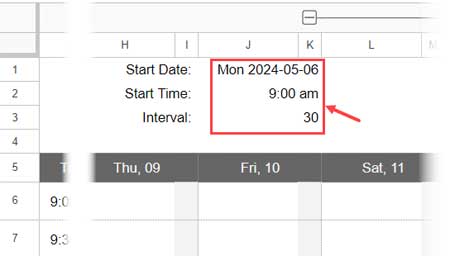
- Set Up Initial Parameters: Enter the start date, start time, and time interval in seconds in cells J1, J2, and J3, respectively.

- Hide Weekend Columns (Optional): If your start date begins on Monday, the template displays time slots for Monday to Sunday. If you wish to hide the Saturday and Sunday columns, click the “-” group sign above column letter K.
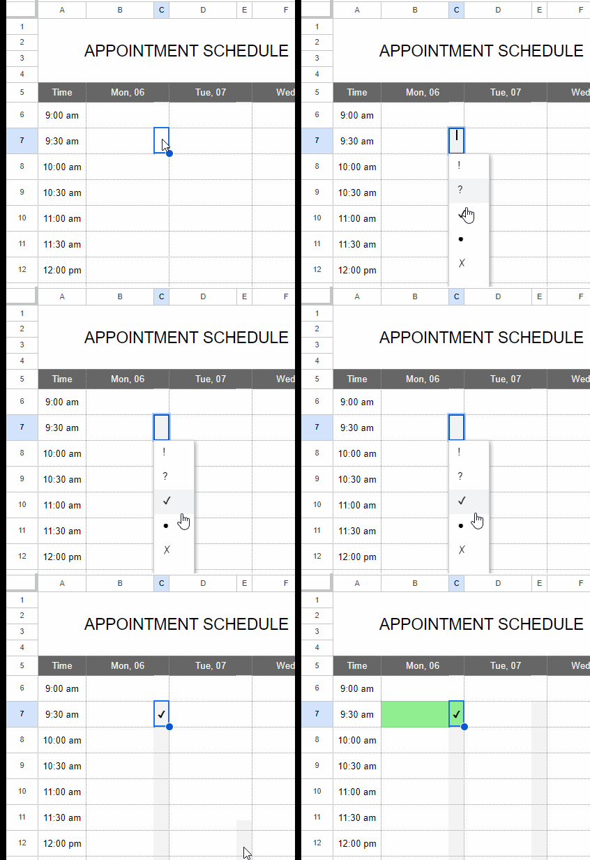
- Color Code Appointments: You’ll find a shaded area within each time slot. Double-click on it and select a symbol to color-code the appointment based on its nature.

Refer to the legend in cells R7:S12 to understand the meaning of each symbol (special character). - Customize Symbols and Text: You may substitute the symbols and relevant text in cell range R7:S12 with your custom symbols and texts. These modifications will be automatically reflected in the time slot drop-downs.
- Adjust Color Coding: If you wish to change the color scheme, click any cell within the time slots (B6:O30) and navigate to Format > Conditional formatting.
- Hide Additional Columns for Printing: Before printing the template, click the “-” group button above column letter “P” to hide columns Q and R.
- Duplicate Weekly Tabs: Each week, duplicate the tab by right-clicking the tab name and selecting “Duplicate.” Then delete everything in the timeslot area.
By following these steps, you can effectively use this appointment schedule template in Google Sheets to organize your appointments and manage your time efficiently.
Understanding the Formulas
The appointment schedule template relies on two array formulas: one in cell B5 and the other in cell A6.
The B5 formula generates a sequence of dates starting from the specified start date in cell J1 and spanning seven days ahead.
Formula #1:
=ArrayFormula(LET( start, J1, m_cells, 2, n, 7, seq, SEQUENCE(1, n*m_cells, m_cells)/m_cells, IF(MOD(seq, 1)=0, start+seq-1, " ") ))The formula employs the LET function to define variables and simplify the expression. It calculates a sequence of dates by incrementing the start date by one day at a time for seven days. Despite the merged cells in B5:O5, the formula accurately returns the sequence of dates only in the visible cells. You can learn more about this technique in my tutorial “Creating Sequential Dates in Equally Merged Cells in Google Sheets“.
The A6 formula generates time slots based on the interval specified in cell J3, starting from the time specified in cell J2.
Formula #2:
=ArrayFormula(J2+time(0, SEQUENCE(25, 1, 0, J3), 0))This formula utilizes the SEQUENCE function to create a sequence of numbers representing minutes, which is then converted into time slots by adding them to the start time specified in cell J2. You can find more details about this formula, or a similar one, in my tutorial “How to Increment Time By Minutes and Hours in Google Sheets“.
Drop-downs and Highlight Rules in the Appointment Schedule Template
The drop-downs in the shaded area utilize the special characters in the range R7:R12.
There are six highlight rules in this appointment schedule template. To view them, click any cell in the time slot and navigate to Format > Conditional formatting.
Let’s analyze one of them: =OR(B6=$R$7, OFFSET(B6, 0, 1)=$R$7)
This formula tests whether the special character in cell R7 matches the special character in cell B6 or C6. If either condition is met, the formula returns TRUE, resulting in both the cells being highlighted.
In this formula, R7 is an absolute reference, while B6 is a relative reference. Thus, as the formula evaluates all cells in the range, R7 remains constant.
Resources
Here are a few more free Google Sheets templates along with usage instructions.


