Using the AND, OR, and NOT logical functions in conditional formatting is useful for creating clever formatting rules in Google Sheets.
The essence of conditional formatting is criteria-based highlighting of a cell or cell range, making these logical functions essential.
Through conditional formatting, we can visualize Gantt Charts, Heat Maps, and more. It’s also useful for easily identifying duplicates in spreadsheets.
Additionally, with the ‘Filter by color’ or ‘Sort by color’ options in the Data menu filter, we gain another advantage: the ability to filter or sort conditionally formatted cells.
While there may be more benefits to conditional formatting, I primarily utilize it in Google Sheets for the purposes mentioned above.
This tutorial elaborates on how to use AND, OR, and NOT in conditional formatting. I will demonstrate how to use these functions individually in formulas.
Sample Data
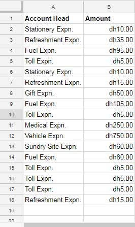
The sample data includes various account heads in column A and their corresponding expenses in column B. The data range spans from A1 to B18.
Since the titles are located in A1 and B1, the “Apply to range” for conditional formatting will be A2:A18, B2:B18, or A2:B18.

Using the OR Logical Function in Conditional Formatting
In the above sample data, column A covers the daily expenses of one of our salespeople. Specifically, I want to highlight only the “Fuel Expn.” and “Toll Expn.” accounts.
Conditional Formatting Formula using OR:
=OR($A2="Fuel Expn.", $A2="Toll Expn.")Syntax:
OR(logical_expression1, [logical_expression2, …])Where:
logical_expression1:$A2="Fuel Expn."logical_expression2:$A2="Toll Expn."
To apply:
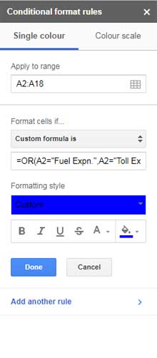
Select the range A2:A18 and then click Format > Conditional Formatting. Under Format Rules, select “Custom formula is”.
Copy-paste the above formula in the given field, choose a formatting style, and click Done.

FAQs:
How can I highlight both columns if one of the specified conditions is met, such as when the OR function evaluates to TRUE?
No changes need to be made to the formula. Simply specify the range correctly. In our case, replace the “Apply to range” from A2:A18 with A2:B18. That’s it.
How do I add more conditions to the OR test?
You can add more logical expressions by separating each one with a comma. For example, to highlight rows containing “Fuel Expn.”, “Toll Expn.”, and “Refreshment Expn.”, use this formula: =OR($A2="Fuel Expn.", $A2="Toll Expn.", $A2="Refreshment Expn.")
Using the NOT Logical Function in Conditional Formatting
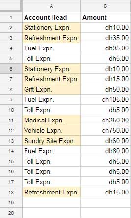
The purpose of using the NOT logical function is essentially the opposite of using the OR logical function in highlighting.
I am using the following formula to highlight cells in the range A2:A18 where the text strings are not “Fuel Expn.” or “Toll Expn.”.
Conditional Formatting Formula using NOT:
=NOT(OR($A2="Fuel Expn.", $A2="Toll Expn."))Syntax:
NOT(logical_expression)Where:
logical_expression:OR($A2="Fuel Expn.", $A2="Toll Expn.")
When you compare the above formulas, you can find the similarity that the same first OR formula is used here but wrapped with NOT.
This formula highlights the cells in A2:A18 if they do not match “Fuel Expn.” or “Toll Expn.”
The FAQs are applicable here as well, i.e., highlighting the entire row and adding more logical expressions.

Using the AND Logical Function in Conditional Formatting
In the use of AND, OR, and NOT in conditional formatting, understanding OR and NOT is straightforward. However, utilizing AND in the highlighting rule presents a different approach. Unlike the former two, the AND function typically involves conditions from two or more columns.
Let’s consider the expense data again. Suppose I want to highlight the cells in the range A2:A18 if the text string is “Fuel Expn.” (in column A) and the corresponding amount (in column B) is greater than or equal to 100.
Conditional Formatting Formula using AND:
=AND($A2="Fuel Expn.", $B2>=100)Syntax:
AND(logical_expression1, [logical_expression2, …])Where:
logical_expression1:$A2="Fuel Expn."logical_expression2:$B2>=100
The FAQs under the OR Logical function are applicable here as well.
AND Function in Highlighting and Two or More Criteria from the Same Column
Time to wrap up this tutorial. However, I believe there’s one clarification needed. I previously mentioned that the “AND” function typically involves conditions from two or more columns. But there are exceptions.
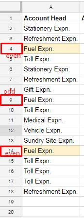
Here’s an example illustrating the use of the “AND” function within the same column in a conditional formatting rule:
In this example, I’m highlighting text in column A if it’s equal to “Fuel Expn.” and appears in even rows.
Formula:
=AND($A2="Fuel Expn.", ISEVEN(ROW($A2)))
That’s all about the use of AND, OR, and NOT in conditional formatting in Google Sheets.
Resources
- Combined Use of IF, AND, and OR Logical Functions in Google Sheets
- How to Use AND and OR with the Google Sheets FILTER Function
- How to Correctly Use AND and OR Functions with IFS in Google Sheets
- How to Use IF, AND, and OR with Arrays in Google Sheets
- Comparison Operators in Google Sheets and Equivalent Functions
- How to Use And, Or, and Not in Google Sheets Query


I would like to highlight a row based on a cell in the row having at least one of two specific words.
Hi, Gary,
You can use Regexmatch. Here is an example (and also check my answers to other comments).
=regexmatch(D8,"(?i)apple|orange")It will return TRUE either apple or orange is present.
This is very helpful. Thank you.
Can you do a cell reference, to a cell with a logical operator in it, within conditional formatting?
For instance, you want to test =A1>A3, but rather than typing the > directly into the conditional formatting formula, you have a > in cell A2.
This way, the user can see what logical operator is being used for conditional formatting and change it if needed.
So the conditional formatting formula would be something like
=A1&A2&A3or maybe=A1&"A2"&A3. But these do not work.Do you know how to accomplish this?
Hi, Doug,
We can accomplish this using a Query.
=ifna(query({A1,TRUE},"Select Col2 where Col1"&A2&A3&"",0),FALSE)In cell A2, feel free to enter any comparison operators. But do remember to put an apostrophe when using the
=sign.I used this formula, but Google Sheet says it is invalid.
=AND(S3="Worse", R3=>0.01)Hi, Elmer Dalangin,
It should be
=AND(S3="Worse", R3>=0.01)Just wanted to say thanks. This helps a lot.
My students can answer 3, 6, or 9. I want to turn all cells red in that column with answers that are NOT 3, 6, or 9. (My first row of data is row 4 in column CG)
I tried this:
=NOT(OR(CG4="3",CG4="6",CG4="9"))But it’s not working. Any ideas what I’m doing wrong?
Hi, Angela Duper,
You have specified the numbers as text strings.
You can try this.
=NOT(OR(CG4=3,CG4=6,CG4=9))How do you format 3 consecutive rows based on the value of one of them? I have multiple (same style) headers on a dispatch spreadsheet that I would like to be able to color format based on their status. I can do/have done it for individual lines, but I’m stuck on how to do it for 3 consecutive rows. I can provide an example if needed. I just would not prefer to post my sheet
Hi, ryan,
Feel free to share the sheet. I won’t publish that comment/reply.
How would this work with checkboxes?
Normally I would do something like:
=COUNTIF($E2, "=TRUE")to format a box based on a checkbox, but I’m currently trying to do an AND statement in this scenario:
Both F2 and G2 have checkboxes. I want G2 to turn red if F2 is true AND G2 is false. How might I accomplish this?
Thanks!!
Hi, Christopher Slagel,
Instead of Countif, you can simply use the formula
$E2=TRUE.Regarding your new requirement, I mean the AND use, use this one.
=and(F2=TRUE,G2=FALSE)Is it just I or the separator between conditions when using the custom formula should be a semicolon ‘;’ instead of a comma ‘,’? In my case I couldn’t enter the ‘,’ between elements in a condition.
Please refer to Regional Settings.
Hi,
Is it possible to refer the A2 in your example to a list of words?
=OR(A2="Fuel Expn.",A2="Toll Expn.")Hi, Loe,
It’s possible not with OR logical function but with REGEXMATCH.
Here is the alternative to the formula you have quoted in your comment.
=not(regexmatch(A2,"Fuel Expn.|Toll Expn."))To use it in a list follow the below example.
If I have my list in D2:D3 (D2 contains “Fuel Expn.” and D3 contains “Toll Expn.” I can rewrite the formula as below.
=not(regexmatch(A2,textjoin("|",true,$D$2:$D$3)))Replace $D$2:$D$3 with the range containing your list.
Best,