")


")


")

")
")
 in Excel & Google Sheets")


Do you want to search for a value selected from a drop-down in an Excel table and filter the headers—specifically, the first row and column? This tutorial provides a solution tailored for Excel users looking to search data in tables and dynamically filter based on selections.
This tutorial introduces a powerful Excel formula technique that utilizes Excel’s dynamic array functionality, making it compatible with Excel 365.
Do you know how this can be a very useful Excel formula? Let me explain the concept first.
For example, in a school timetable with days of the week in the top row, timeslots in the first column, and subjects within the grid, you can search for a subject and return the timeslots and names of the weekdays from the table.
See the table below:
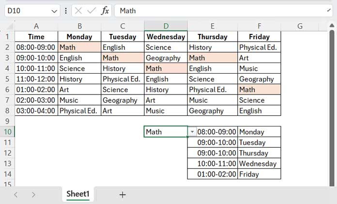
In this table, if you search for ‘Math’ within the grid, it will return the corresponding names of the weekdays from the header row and timeslots from the first column. This allows students or teachers to know on which days this subject is scheduled and at what times.
Here are step-by-step instructions to interactively search tables in Excel and return headers from the table.
Identifying Search Values and Table Headers
In the table above, B2:F8 represents the range containing various subject names that we want to search for.
The range B1:F1 represents the headers, which are the days of the week that we want to filter, and A2:A8 contains the timeslots associated with each day.
So, if you search for the subject “Math,” the formula should return the day of the week the subject is scheduled as well as the corresponding timeslots.
This means the formula will search for a value in the table and return both the header and the first column. The search process will be interactive using a drop-down menu to switch between subjects.
Create a Drop-Down Menu for Interactive Filtering in Excel
To create a drop-down menu to search for a value within the table, follow these steps in Excel:
- Enter the following formula in an empty column, for example, in cell O2:
=LET(value_range,B2:F8,UNIQUE(TOCOL(value_range)))
Where B2:F8 contains the values that you want to search for. This formula returns the unique values in this range in a column. - Navigate to any cell where you want to create the drop-down menu. For example, let’s choose cell D10.
- Click on the Data tab, and within the Data Tools group in the ribbon, click Data Validation.
- In the Data Validation dialog box, under Settings > Validation Criteria > Allow, select List.
- In the Source field, select O2:O9, which is the output returned by the formula in step 1.
- Click OK. Your data validation drop-down menu is now ready. You can select values from this drop-down to dynamically filter the table header and first column.
Now, let’s see how to search for values selected from this drop-down menu within the table grid and return the corresponding headers and the first column.
Search by Value and Filter Headers & First Column
Next to the drop-down menu, i.e., in cell E10, enter the following formula which searches the table and filters the headers based on the drop-down selection:
=LET(unpivot, REDUCE(HSTACK("Title1","Title2","Title3"),TOCOL(A2:A8&"|"&B1:F1&"|"&B2:F8),LAMBDA(a,v,VSTACK(a,LET(ts,TEXTSPLIT(v,"|"),IFERROR(ts*1,ts))))),FILTER(CHOOSECOLS(unpivot,{1,2}),CHOOSECOLS(unpivot,3)=D10))Where:
A2:A8: Values to filter in the first column.B1:F1: Headers to filter in the first row (header row).B2:F8: The grid (search range).D10: The value in the drop-down menu to search within the grid.
Please note the following:
- The number of rows in the first column (A2:A8) must match the number of rows in the search grid (B2:F8).
- The number of columns in the header row (B1:F1) must match the number of columns in the search grid (B2:F8).
This formula returns the headers (days of the week in the header row) and values in the first column (timeslots) corresponding to the value selected in the drop-down menu in cell D10.
Formula Deep Dive: Enabling Dynamic Header & Column Filtering
This section is optional for those who just want to use the formula without an in-depth explanation.
We used the Excel LET function to name and define a value expression, which we then used within the formula to simplify and enhance its performance.
Syntax of the LET Function in Excel:
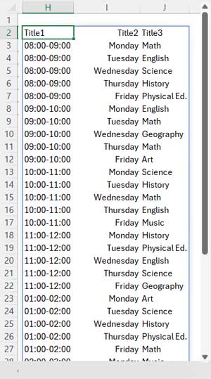
LET (name1, name_value1, [name2], [name_value2], …, calculation)name1:unpivotname_value1:REDUCE(HSTACK("Title1","Title2","Title3"),TOCOL(A2:A8&"|"&B1:F1&"|"&B2:F8),LAMBDA(a,v,VSTACK(a,LET(ts,TEXTSPLIT(v,"|"),IFERROR(ts*1,ts)))))
This formula unpivots the data, as detailed in my tutorial titled “Unpivot Excel Data Fast: Power Query & Dynamic Array Formula.”
Result:
calculation:FILTER(CHOOSECOLS(unpivot, {1, 2}), CHOOSECOLS(unpivot, 3) = D10)
The FILTER function filters the first and second columns in the unpivoted data based on the search key in the third column.
This allows us to dynamically filter the header row and first column based on a value in the table grid in Excel.
Error Handling
The formula that searches the table and filters headers, not the formula used for the drop-down, may return the following two errors:
#CALC!: Occurs when the search key is empty or doesn’t match any value in the grid.#N/A: Occurs when the dimensions of the specified headers, first column, and search ranges do not match, as explained previously.
These errors can help identify issues with the formula’s inputs or configuration in Excel.