


We can flip a table vertically in two ways in Excel: by reversing the row order of the original table or by using a formula. It’s worth noting that the formula will generate a new dataset from the source table. This tutorial covers both methods.
There are several reasons one might consider flipping a table vertically in Excel. For instance, imagine you have a table in Excel containing data arranged in chronological order but lacking a date column. In such a scenario, flipping the rows in the table vertically can assist in placing the latest data at the top.
Flipping the Source Table Vertically in Excel
We will apply this to a small table in the range A1:C5 to illustrate correctly. I’ve organized the steps into two categories:
- Steps (for table) – Applicable to a formatted table
- Steps (for range) – Applicable to a data range.
Steps (for table)
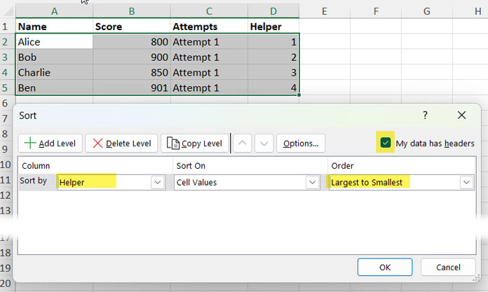
- In cell D1, enter the label ‘Helper’.
- In cells D2:D5, enter sequential numbers from 1 to 5. You can start with 1 in D2, then 2 in D3, and drag the fill handle at the bottom right corner of cell D3 down to D5 to fill the series.
- The table should already be expanded to A1:D5. If not, click anywhere in the table, go to the Table Design menu, then click on Resize Table in the Properties group. Select A1:D5 and click OK.
- Click the drop-down arrow in cell D1 and choose “Sort Largest to Smallest”.
- Delete the helper column.
This is one of the simplest methods to flip a table vertically in Excel.
Steps (for range)
If you are using the range A1:C5 instead of a table, you can skip the third step above. In the fourth step, select range A1:D5, click on the Data menu, then go to Sort in the Sort & Filter group, and sort the data by the fourth column (Helper) from largest to smallest.
This way, we can flip a data range vertically without using any formula in Excel.
Vertically Flip the Table Using a Formula (Dynamic or Non-Dynamic)
If you prefer not to modify your source table and instead create a new flipped table in Excel, you can utilize the following formula approaches. The helper column used in the previous examples is not required here.
Non-Dynamic (OFFSET-based)
In cell E2, enter the following formula:
=OFFSET($A$2, ROWS(A2:$A$5)-1,,,3)Then, select the fill handle and drag it down until cell E5.
How does this formula flip the table vertically in an Excel spreadsheet?
The formula employs the OFFSET function with the syntax: OFFSET(reference, rows, cols, [height], [width]).
Where:
referencerefers to the first cell in the table, excluding the header row, which is A2.rowsrepresents the number of rows to shift from cell A2, denoted asROWS(A2:$A$5)-1cols,heightare omitted.widthis set to 3, representing the total number of columns in the table.
When you drag the fill handle down, ROWS(A2:$A$5)-1 becomes ROWS(A3:$A$5)-1, ROWS(A4:$A$5)-1, and ROWS(A5:$A$5)-1, resulting in 3, 2, 1, and 0 as the number of rows to shift, respectively.
Dynamic Array Formula (SORTBY-based) to Vertically Flip a Table in Excel
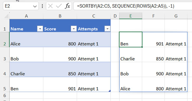
Alternatively, for a dynamic solution without relying on a non-dynamic formula, consider the following SORTBY-based formula:
=SORTBY(A2:C5, SEQUENCE(ROWS(A2:A5)), -1)Note: This formula will only work in Excel versions that support the SORTBY and SEQUENCE functions.
Syntax:
SORTBY(array, by_array1, [sort_order1], [by_array2, sort_order2],…)Where:
arrayrefers to A2:C5, indicating the table range excluding the header row.by_array1isSEQUENCE(ROWS(A2:A5)), which returns sequence numbers corresponding to the size of the first column in the array.sort_order1is -1, instructing to sort the table in descending order based on values inby_array1.
When using formulas (whether they are dynamic arrays or not) to flip a table in Excel, any changes made to the source table will be reflected in the result. Additionally, editing the result directly may break the formula.
If you don’t want this behavior, select the result, right-click to open the context menu, choose ‘Copy,’ then right-click again to open the context menu, and select ‘Paste Special’ > ‘Paste Values’.
Resources
You can vertically flip a table in several ways in Excel. The above are the two best options that even newbies can consider. Here are a few more Excel resources.