


This post is specific to using Not in Regexmatch in Google Sheets.
In some cases, we can use alternatives, such as Find, Search, and Match with wildcards, to Regexmatch in Google Sheets.
So I have included how to use Not in Regexmatch and its alternatives using Find (case-sensitive) and Search (case-insensitive).
Learning RE2 regular expressions and their use in Google Sheets is not much hard as you think.
What you may want to do is to try it first with some basic examples. You can find some in my REGEXMATCH tutorial.
How to Use NOT in REGEXMATCH in Google Sheets
We can’t negate a piece of text using the expression (?!) in Regex in Google Sheets as it’s not supported.
The alternate way is using the NOT logical operator in Regexmatch in Google Sheets.
Assume I want to check whether cell D25 doesn’t contain the word “inspiration.”
The below formula in any other cell will do the test and return TRUE or FALSE Boolean values.
Formula 1:
=not(regexmatch(D25,"(?i)inspiration"))If it returns TRUE, it simply means the text “inspiration” is not present in cell D25.
The above is a case-insensitive Regexmatch formula. To make it case-sensitive, use the below one.
Formula 2:
=not(regexmatch(D25,"inspiration"))Alternatives Using NOT Find and NOT Search
The above two formulas show how to use NOT in Regexmatch in Google Sheets using RE2 regular expressions and a logical function.
Here is my attempt to replace the regular expression with the functions Find and Search.
To replace formula 1, we should use the SEARCH with Not as below. That means the below formula is case-insensitive.
=not(len(iferror(search("inspiration",D25))))To replace formula 2 with its alternative, just substitute “search” with “find.”
=not(len(iferror(find("inspiration",D25))))Can you explain the above two formulas?
Yep! FIND (also Search) returns the position at which a string is first found within D25.
It will return ‘#VALUE!’ when the string “inspiration” is not present in D25.
You may already know the use of the IFERROR function. Here it makes an error to blank.
The LEN returns the length of the characters that are returned by IFERROR(FIND/SEARCH).
The Len, i.e., LEN(IFERROR(FIND/SEARCH)), will return FALSE if the length is blank.
What we want is TRUE when there is no match or we can say the length is blank. There comes the use of Not, i.e., NOT(LEN(IFERROR(FIND/SEARCH))).
I hope the above makes sense.
NOT in REGEXMATCH Array Formulas in Google Sheets
We can use all the above Not in Regexmatch and alternative formulas in a range/array with the help of the ARRAYFORMULA function.
Please see the following screen capture. There are four array formulas in cell range E25:H25, and here are them.
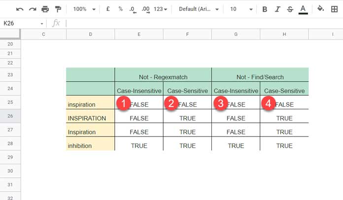
E25:
=ArrayFormula(not(regexmatch(D25:D28,"(?i)inspiration")))F25:
=ArrayFormula(not(regexmatch(D25:D28,"inspiration")))G25:
=ArrayFormula(not(len(iferror(search("inspiration",D25:D28)))))H25:
=ArrayFormula(not(len(iferror(find("inspiration",D25:D28)))))Please also check the titles in cell range E24:H24.
Match and Does Not Match in a Single Regexmatch Formula
I want to test a cell in the following way.
Check item “apple” is present and “mango” is not present in cell D3. How do I test it?
It’s so simple. We can use all the above four formulas. I mean two Not in Regexmatch and two of its alternatives.
How?
Syntax (Using Regexmatch): =regexmatch_formula*not(regexmatch_formula)
Formula 1:
=regexmatch(D3,"(?i)apple")*not(regexmatch(D3,"(?i)mango"))Formula 2:
=regexmatch(D3,"apple")*not(regexmatch(D3,"mango"))Syntax (Alternatives): =len(iferror(search_or_find))*not(len(iferror(search_or_find)))
Formula 1:
=len(iferror(search("apple",D3)))*not(len(iferror(search("mango",D3))))Formula 2:
=len(iferror(find("apple",D3)))*not(len(iferror(find("mango",D3))))Note:- The above formulas return 1 or 0 instead of TRUE or FALSE. I hope you can easily convert them to Boolean values.
Can we use them in array formulas? Yep! Here you go!
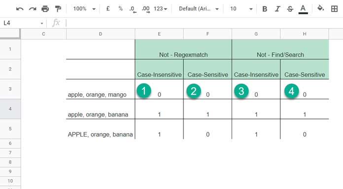
Formulas in E3:H3 are as follows.
E3:
=ArrayFormula(regexmatch(D3:D5,"(?i)apple")*not(regexmatch(D3:D5,"(?i)mango")))F3:
=ArrayFormula(regexmatch(D3:D5,"apple")*not(regexmatch(D3:D5,"mango")))G3:
=ArrayFormula(len(iferror(search("apple",D3:D5)))*not(len(iferror(search("mango",D3:D5)))))H3:
=ArrayFormula(len(iferror(find("apple",D3:D5)))*not(len(iferror(find("mango",D3:D5)))))This way we can use Not in Regexmatch in Google Sheets.
That’s all. Thanks for the stay. Enjoy!