


![Excel Hotel Room Availability Template [Free]](https://infoinspired.com/wp-content/uploads/2024/05/Excel-Hotel-Room-Availability-Template-218x150.jpg "Excel: Hotel Room Availability and Booking Template (Free)")


This post explains how to filter the top 3 most frequent strings in Google Sheets.
Before going to an example, let me clarify one important point about the result that my formula will return.
Assume there are five strings, and the occurrences of them are as follows.
| Values | Number of Times (Occurrences) |
| A | 4 |
| B | 1 |
| C | 4 |
| D | 5 |
| E | 2 |
Note:- For the sample data, please jump to image # 1 below (A2:A). We will find the occurrences as above using a COUNTIF later.
My formula is going to return the strings D (5 occurrences), A (4 occurrences), C (4 occurrences), and E (2 occurrences).
We want three strings, right? Then why does the formula return four strings?
It is because there are two strings in the second position, and they are A and C with four occurrences each.
One more thing!
Earlier, we have learned how to find the MODE of text values.
That post is related to finding the top most frequent string (MODE) / strings (MODE.MULT), not about finding the top 3 or n most frequent strings.
I’ll explain step by step how to filter the top 3 most frequent strings in Google Sheets.
Please note that you can use ‘n’ instead of 3 without making any major changes in the formula.
Example
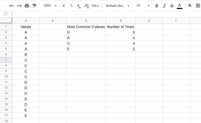
In the above example, the sample texts are in A2:A, and my formula in C2 returns the most frequent three values and their occurrences in the number of times.
As you can see, the formula returns four values since the values “A” and “C” repeat twice, which I have already explained above.
Let’s go to the tutorial section.
Filter the Top 3 Most Frequent Strings in Google Sheets
We will use a few helper columns (additional columns) in the beginning steps, and on the course, we can remove those.
There are three main steps involved. Here are them.
Step # 1 – COUNTIF Array to Return the Count of Strings
Prepare a sample sheet as per the above image. Just enter the values in A2:A. Leave other values.
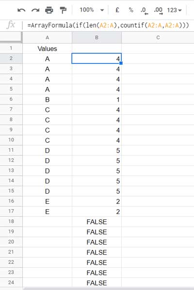
In that sheet, in cell B2 insert the below COUNTIF Array Formula to return the count of text strings in A2:A.
=ArrayFormula(if(len(A2:A),countif(A2:A,A2:A)))To make you know what the COUNTIF returns, I am leaving the corresponding screenshot below.
In the above formula, you may want to know the LEN use. You can find that here – LEN Function in Google Sheets and Practical Use of It.
The COUNTIF returns how many times each string occurs.
Step # 2 – Find the Number of Times the Most Frequent N Strings Occur
The next two Google Sheets formulas determine the number of most frequent strings that you want to filter.
First, you may enter the below SORTN, UNIQUE, and COUNTIF combination formula in cell D2.
=sortn(unique(countif(A2:A,A2:A)),3,0,1,0)Formula Explanation
The COUNTIF enclosed within UNIQUE returns the unique values from the values in column B.
In the above formula, instead of referring to the COUNTIF result in B2:B, I have used the same formula within the UNIQUE itself.
The 3 in SORTN means return 3 values after sorting column 1 (there is only one column) in descending order.
If you want to filter the top 5 most frequent strings in Google Sheets, change 3 to 5 in the formula.
SORTN Explained Further
Now I am talking about the 0 present after the 3. It’s one of the SORTN display_ties_mode. It determines what to do in case of duplicates.
If you want, you can read more about ties mode here – SORTN Tie Modes in Google Sheets – The Four Tiebreakers.
The next 1 indicates the sort column, and 0 means to sort the column in descending order (Z-A).
Step # 2.1 – Coding a Regular Expression to Filter the Most Frequent 3 Strings
Now I am coming to the logic of my final formula that you will get after one more step below. So please pay extra attention.
Logic
We will filter the strings in A2:A based on the number of times they appear. But not just based on the number of times, but based on the top n number of times returned by the step # 2 formula.
So we will use the FILTER function to filter A2:A if B2:B (COUNTIF Array) values are equal to Step # 2 result.
To specify B2:B is equal to Step # 2 result in FILTER, we can use the REGEXMATCH in FILTER as below.
Generic Formula (You will get the final formula based on this generic formula in the next step)
=FILTER(A2:A,regexmatch(B2:B&"",step_2.1_formula))Now, first, let’s understand the REGEXMATCH formula within the above Generic Formula.
The REGEXMATCH is one of the Text functions in Google Sheets. Since B2:B contains numbers, I’ve converted them to text by adding a null character. I mean B2:B is replaced by B2:B&"".
Otherwise, REGEXMATCH will return #VALUE! error stating something similar below.
Function REGEXMATCH parameter 1 expects text values. But ‘5’ is a number and cannot be coerced to a text.
Then what is the step_2.1_formula?
To match multiple numbers, in REGEXMATCH, we should combine the numbers in a specific way as below. That’s the step # 2.1 formula (a modified version of the D2 [Step # 2] formula).
="^"&textjoin("$|^",true,sortn(unique(countif(A2:A,A2:A)),3,1,1,0))&"$"The above is as per the below generic formula.
="^"&textjoin("$|^",true,step_2_formula)&"$"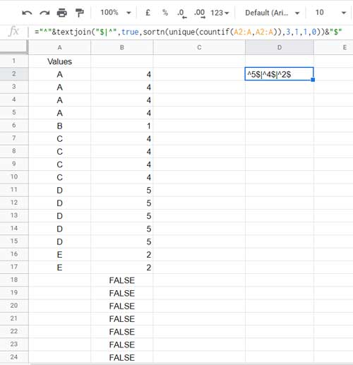
Time to filter the most frequent 3 strings using the above number of times.
Step # 3 – Filter the Most Frequent 3 Strings Using Number of Times (Step 2.1 Result)
Once again, please pay attention to the generic formula to filter the most frequent 3 strings in Google Sheets.
=FILTER({A2:A,B2:B},regexmatch(B2:B&"",step_2.1_formula))I’ve already explained all the required parameters to use in the FILTER. So I am going straightaway to the formula (not to the final formula).
Copy-paste the above generic formula to cell C2. Cut D2 formula (step_2.1_formula) and replace step_2.1_formula in the C2 generic formula with that.
Formula
=filter({A2:A,B2:B},regexmatch(B2:B&"","^"&textjoin("$|^",true,sortn(unique(countif(A2:A,A2:A)),3,1,1,0))&"$"))It’s high time to remove the helper columns. For that, replace B2:B (it appears twice in the formula) with the formula in B2 itself.
=filter({A2:A,if(len(A2:A),countif(A2:A,A2:A))},regexmatch(if(len(A2:A),countif(A2:A,A2:A))&"","^"&textjoin("$|^",true,sortn(unique(countif(A2:A,A2:A)),3,1,1,0))&"$"))Finally, you may enclose this formula with the UNIQUE to remove duplicates (multiple occurrences of rows).
=unique(filter({A2:A,if(len(A2:A),countif(A2:A,A2:A))},regexmatch(if(len(A2:A),countif(A2:A,A2:A))&"","^"&textjoin("$|^",true,sortn(unique(countif(A2:A,A2:A)),3,1,1,0))&"$")))Then SORT the second column in descending order.
=sort(unique(filter({A2:A,if(len(A2:A),countif(A2:A,A2:A))},regexmatch(if(len(A2:A),countif(A2:A,A2:A))&"","^"&textjoin("$|^",true,sortn(unique(countif(A2:A,A2:A)),3,1,1,0))&"$"))),2,0)That’s all. Thanks for the stay, enjoy!