


")


")


How to split or separate numbers from a text string without delimiters by using substrings as delimiters in Google Sheets?
If a delimiter, such as a space character, is present in the text to separate a number, we can use the SPLIT function to separate the number from the text.
But how can we split a number from text when there is no delimiter in Google Sheets?
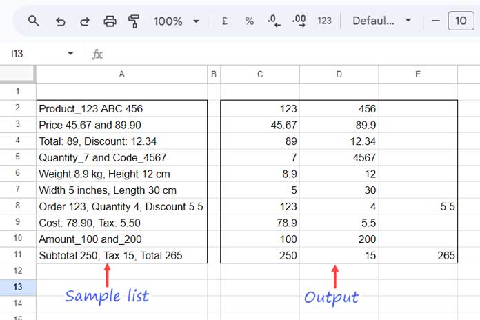
In the list below (range A2:A11), the text strings do not have any common delimiters to separate the numbers from the text.
Since we can’t use the SPLIT function directly, we first need to insert a delimiter using a formula. In Google Sheets, we can achieve this with the REGEXREPLACE function, and then apply the SPLIT function.
Splitting Numbers from Text Without Delimiters in Google Sheets Involves Two Steps:
- Substitute text with a delimiter, leaving the numbers untouched using REGEXREPLACE.
- Split the modified text using the SPLIT function.
We will combine these two steps.
Step 1: Replacing Text with Commas to Facilitate Splitting Without Existing Delimiters
We may encounter various text strings that contain numbers. The numbers could appear at the beginning, middle, or end of the text, and there may be multiple separate numbers within a single string. You can see examples of this in the list (A2:A11) above.
We will convert all non-numeric characters to commas, leaving only numbers and commas in the text.
For the text in cell A2, such as Product_123 ABC 456, use the following REGEXREPLACE formula in cell C2 to insert comma delimiters around the numbers:
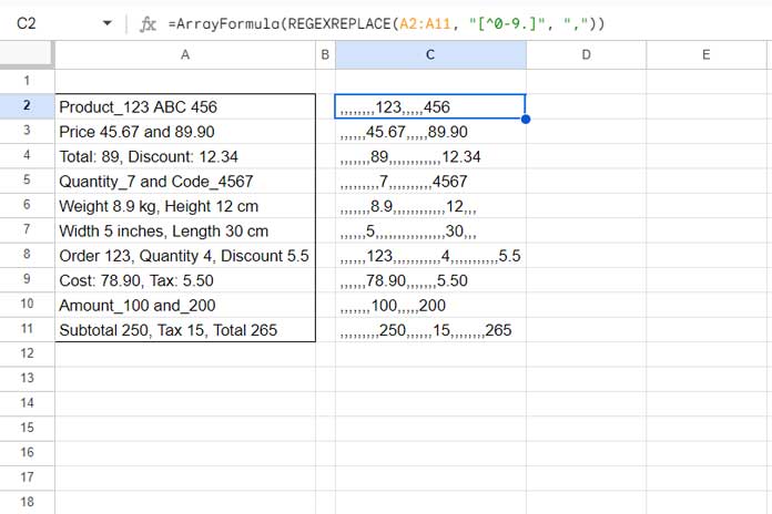
=REGEXREPLACE(A2, "[^0-9.]", ",") // returns ,,,,,,,,123,,,,,456To apply this to the range A2:A11, use the following REGEXREPLACE formula as an array formula:
=ArrayFormula(REGEXREPLACE(A2:A11, "[^0-9.]", ","))In this formula:
"[^0-9.]": This pattern matches any character that is not a digit (0-9) or a dot (.).",": The replacement string.
This method allows us to insert comma delimiters into text strings to separate numbers from text in Google Sheets.
The output will look like this:
Step 2: Separating Numbers from Text
We’ve inserted delimiters in the previous step. Now, how do we separate the numbers?
If you’re referencing a single cell, such as cell A2, you can wrap the REGEXREPLACE function with the SPLIT function as follows:
=IFERROR(SPLIT(REGEXREPLACE(A2, "[^0-9.]", ","), ",", ,TRUE))This will separate the numbers. For example, if you enter the formula in cell C2, the result will appear across cells C2, B2, and so on.
Note that if cell A2 is empty, the formula will return an empty result due to the use of IFERROR.
To apply this to the range A2:A11, use the following array formula in cell C2:
=ArrayFormula(IFERROR(SPLIT(REGEXREPLACE(A2:A11, "[^0-9.]", ","), ",", ,TRUE)))This method allows us to separate numbers from text even when no delimiter is initially present.
Splitting Numbers from Text While Retaining Both
Previously, we discussed how to split numbers from text, which actually separates the numbers. If you want to split each number in the text while keeping both numbers and text, use the following formulas:
For cell A2;
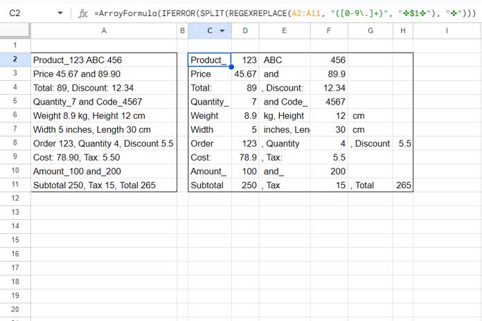
=IFERROR(SPLIT(REGEXREPLACE(A2, "([0-9\.]+)", "✜$1✜"), "✜"))For the range A2:A11:
=ArrayFormula(IFERROR(SPLIT(REGEXREPLACE(A2:A11, "([0-9\.]+)", "✜$1✜"), "✜")))In this formula:
"([0-9.]+)": The regular expression pattern used to match sequences of digits and dots."✜$1✜": The replacement string.✜is used as a custom delimiter to surround the matched numbers.
Resources
- Extract All Numbers from the Text and Sum Them in Google Sheets
- Sum Cells With Numbers and Text in a Column in Google Sheets
- How to Extract Negative Numbers from Text Strings in Google Sheets
- How to Split a Number into Digits in Google Sheets
- Split to Column and Categorize – Google Sheets Formula
- Split a Column into Multiple N Columns In Google Sheets
- Split a Text after Every Nth Word in Google Sheets (Using Regex and Split)
- Split and Count Words in Google Sheets (Array Formula)
- Split Comma-Separated Values in a Multi-Column Table in Google Sheets
- How to Get the Split Result in Text Format in Google Sheets
- Dynamic Formula: Split a Table into Multiple Tables in Google Sheets
- Split Your Google Sheet Data into Category-Specific Tables
Hi Prashanth,
I would like to request your help with the expected split output. I have attached a link to the data that I am working with.
[URL removed by Admin]
Thank you!
Hi Bahar,
I can’t access your sheet because it is view only and I can’t make a copy of it.
However, I can share the sample text and formula with you:
Sample Text in Cell A1:
3 apple 12 orange 7 pear pt9 2 water melon 43 grape wb7 5 starfruitFormula:
=ARRAYFORMULA(TOCOL(TRIM(SPLIT(REGEXREPLACE(A1,"\s\d+",",$0"),","))))I hope this helps!
Thank you, Prashanth, for always saving my day.
Thanks, a really interesting and useful explanation of a non-trivial problem.