Sum Cells With Numbers and Text in a Column in Google Sheets

Google Sheets considers numbers mixed with text as text only. So, typically, you cannot sum cells with numbers and text in a column in Google Sheets.

If your data entry operator is new to the job, you may encounter situations that test your data manipulation skills. An inexperienced Data Entry Operator (DEO) can cause the following common errors in your spreadsheet.

A common issue you may encounter in your spreadsheet is a column/row or an array that has numbers mixed with text (alphanumeric characters). Usually, you may come across such entries in columns with currency symbols as well as units of measurement.

How do we sum a column with numbers and numbers mixed with text in Google Sheets? Let’s delve into the details.

Error When Summing Cells Containing Numbers and Text in a Column

Can I use the SUM function to sum the values in column C in the following sample data set?

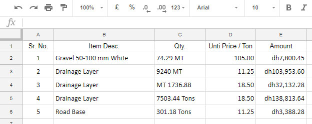
Example to sum cells with numbers and text in Sheets

No, you can’t use the SUM function to sum a column with mixed content as shown below:

=SUM(C2:C6)

The above formula will return 0 because there are no purely numeric values in column C. In column C, all the numbers are mixed with units of measurement, represented as strings/text.

In Google Sheets, to handle such columns with mixed content in calculations, you should first remove the textual parts from the numbers.

Learn how to remove text from numbers in a column and then sum in Google Sheets. It’s not a complicated process.

How to Sum Cells With Numbers and Text in a Column in Google Sheets

Here is the formula to sum a column with mixed content in cells, utilizing Google Sheets functions such as SUM, IFERROR, ArrayFormula, SPLIT, and REGEXREPLACE.

Formula #1 (for a Column):

=ArrayFormula(SUM(IFERROR(SPLIT(REGEXREPLACE(C2:C&"", "[^\d\.]+", "|"), "|"))))

Formula Explanation

We are dealing with an array/range, so we must use the ArrayFormula with other non-array functions in this formula. Now let’s start with the formula explanation step-by-step.

The REGEXREPLACE function replaces all the texts in column C with the pipe “|” symbols.

=ArrayFormula(REGEXREPLACE(C2:C&"", "[^\d\.]+", "|"))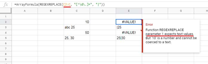

VALUE error in Regex in mixed and alphanumeric column data

Do you know why I have used C2:C&"" instead of C2:C?

This is to convert numbers within the range to text strings. Otherwise, if numbers are present in column C, the formula would return a VALUE! error as the REGEXREPLACE function expects text values in parameter 1.

The SPLIT function splits the above result based on the “|” as the delimiter.

=ArrayFormula(SPLIT(REGEXREPLACE(C2:C&"", "[^\d\.]+", "|"), "|"))

The SPLIT function is not required if you use "" instead of the Pipe symbol in REGEXREPLACE.

I opted to go with the Pipe symbol as sometimes any of the cells may contain multiple numbers as follows: 350 MT, 450 MT

In such a case, if you use "" instead of |, REGEXREPLACE will return this as one whole number like 350450. I want a separator between like 350 | 450 so that I can split it into two separate numbers.

The IFERROR is to remove any other errors associated with blank cells in the column.

=ArrayFormula(IFERROR(SPLIT(REGEXREPLACE(C2:C&"", "[^\d\.]+", "|"), "|")))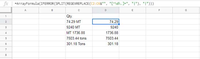

Regex formula to extract numbers from column

Finally, the SUM function sums all the values.

As per our example, if you remove the SUM function from the beginning of the formula, you can use it to extract only numbers from the column. Thus, it can be useful for cleaning your Google Sheets data.

You can use my formula in any column as it’s an array formula. That means this formula can sum an entire column that contains alphanumeric characters. You only need to modify the cell references in this formula to work.

Sum Alphanumeric Characters in a Row in Google Sheets

Can I use the above formula in a row?

Why not? With my formula, you can not only sum cells with numbers and text in a column but also a row. However, you need to tweak the formula a little bit.

If the numbers with text (alphanumeric characters) are in C2:G2, instead of using C2:G2&"", use TRANSPOSE(C2:G2)&"".

Formula #2 (for a Row):

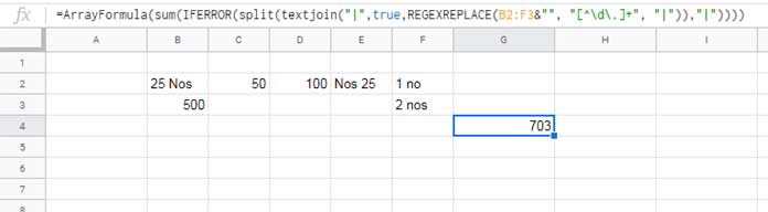
=ArrayFormula(SUM(IFERROR(SPLIT(REGEXREPLACE(TRANSPOSE(C2:G2)&"", "[^\d\.]+", "|"), "|"))))

Here, use the TRANSPOSE function to transpose the row to a column.

Summing Alphanumeric Characters in a 2D Array

To sum alphanumeric characters (cells with numbers and text) in a 2D array, you should tweak the formula #1.

In the following example, I need to sum cells with numbers and text in B2:F3, a 2D array. For that, we need to convert the values into a single column and use our earlier formula.

That means you need to replace C2:C in our formula #1 with TOCOL(B2:F3); the TOCOL function transforms the range of cells into a single column.

Formula #3 (for a 2D Array):

=ArrayFormula(SUM(IFERROR(SPLIT(REGEXREPLACE(TOCOL(B2:F3)&"", "[^\d\.]+", "|"), "|"))))

Note: You can use TEXTJOIN instead of TOCOL.

Sum Cells With Numbers and Text in Multiple Columns

Hope you have learned how to sum a column where numbers are mixed with text in Google Sheets.

Resources

We have used REGEXREPLACE to remove text and facilitate the summation of cells with numbers and text in Google Sheets. Here are some related topics discussing scenarios that involve text, numbers, and summation.

39 COMMENTS

tom September 30, 2024 At 1:46 am

Hey, thanks a lot! I would also like to multiply a cell that contains alphanumeric characters (for example, 400g) by a numeric cell. Would I need to use REGEXREPLACE for that, and how?

- Prashanth KV September 30, 2024 At 7:31 am
  
  You can use either REGEXREPLACE or REGEXEXTRACT to extract the numeric part, then multiply it. Here’s an example that might help:
  
  =REGEXEXTRACT(TO_TEXT(E5),"[\d.]+")*F5
  
  This formula extracts the numeric portion from the text in cell E5 and multiplies it by the value in cell F5
  
  - tom October 1, 2024 At 3:04 am
    
    Thank you!
    
Guilherme February 3, 2024 At 4:44 am

UPDATE: It seems to be working perfectly with this:

=ArrayFormula(SUM(IFERROR(VALUE(REGEXEXTRACT(A2:A30&""; "\d[\d,.]*"))))

- Prashanth KV February 3, 2024 At 5:02 pm
  
  I understand there were two issues. The decimal separator is a comma, not a period in your country. This affects the argument separator in the formula as well. You have addressed both by modifying the regular expression and also the argument separator.
  
  Please check out this: How to Change a Non-Regional Google Sheets Formula.
  
Guilherme February 3, 2024 At 4:09 am

Hello there. I need to be able to sum numbers containing decimals. For example, values “2” and “0.5” should sum up to 2.5 instead of 7. How could I achieve that?

Thanks for your help!

Mike December 25, 2022 At 7:21 pm

Hi Prashanth,

Thanks for sharing this.

I need to know if there is a way, to sum up only cells that match a criterion.

—URL removed by Admin—

Any help would be very appreciated!

- Prashanth December 27, 2022 At 2:57 pm
  
  Hi, Mike,
  
  Please try this formula yourself. I don’t have editable rights to your Sheet.
  
  Replace the range D4:K4 in your formula with if(search("(s)",D4:K4),D4:K4).
  
  So the formula will include the cells containing an “(s)” in them.
  
  Further, you can make a single formula for the whole column. For that, empty the L4:L47 range and insert the following formula in L4.
  
  =byrow(D4:K47,lambda(r,ArrayFormula(SUM(IFERROR(SPLIT( REGEXREPLACE(TRANSPOSE(if(search("(s)",r),r))&"", "[^\d\.]+", "|"), "|"))))))
  
  - Mike December 28, 2022 At 8:54 am
    
    Thank you so much!
    
Mustafa November 28, 2022 At 11:27 am

Dear Prashanth,

Thank you for your simplified solutions

I want to use your Formula # 3 on my sheet on which data is submitted from a Google Form, and I need to automate the results.

Kindly help with this.

Thank you.

- Prashanth November 30, 2022 At 2:11 pm
  
  Hi, Mustafa,
  
  Please feel free to share a Sample Sheet. You can leave it (URL) in the comment below which won’t be posted.
  
Salvatore April 6, 2022 At 6:01 am

Having trouble finding a way to do something similar but not quite this.

On my Master Sheet, I am using Vlookup to find the data from a sheet called Classes.

I’m trying to add two data pulls in one cell. However, it’s not adding correctly or not at all.

So, using J1 and K1 for criteria 1, and L1 and M1 for criteria 2.

The drop-down list in L is set to Class if not used.

The column I’m pulling from has either single numbers or 2 or 3, or 4 numbers separated by a slash ex. +1, +6/+1, +11/+6/+1, +20/+15/+10/+5.

By the way, I had to set that column to text so they wouldn’t auto transform to dates.

I’m trying to have it added together. So that using those examples, it would read +38/+22/+11/+5 in one cell.

Using;

=if($L$1="Class",vlookup($J$1&" "&$K$1,Classes!$B$2:$D,2,false), vlookup($J$1&" "&$K$1,Classes!$B$2:$D,2,false)+vlookup($L$1&" "&$M$1, Classes!$B$2:$D,2,false))

It works if L1 is Class or the numbers are all single numbers.

Any advice?

- Prashanth April 6, 2022 At 11:48 am
  
  Hi, Salvatore,
  
  Please prepare a sample sheet. Then share the URL in the reply below.
  I won’t publish that comment.
  
Imam November 22, 2021 At 10:01 pm

Hi Prashanth,

I have table in sheet with data U2, U, A, U1 in rows. Is it possible to get data sum U = 6 (U + 2 + U + U + 1)
How to create a formula with this case? I think, need to update the regex expression, but I haven’t been able to find a way.

Really appreciate it if you can help me.

Best,
Imam

- Prashanth November 23, 2021 At 11:13 am
  
  Hi, Imam,
  
  It seems possible. Please share a sample of your Sheet.
  
  - Imam November 23, 2021 At 8:00 pm
    
    Hi Prashanth,
    
    Please follow this link — removed by admin —
    
    If you need to edit in Sheet, please share your email.
    
    - Prashanth November 24, 2021 At 8:26 am
      
      Hi, Imam,
      
      Please try this formula for column range D2:D9, i.e., for November.
      
      =ArrayFormula(sum(split(filter(regexreplace(D2:D9&"","U","1|"), regexmatch(D2:D9,"U")),"|")))
      
      Change “U” to “A”
      
Tyler November 22, 2021 At 9:50 pm

Totally makes sense! The array approach looks extremely versatile. I hope to dive deeper into that one soon. Many thanks!!

Tyler November 17, 2021 At 8:45 pm

I have a similar question to Ella from above. Firstly, thank you for your explanations. They’re great.

I have cells with numbers, letters, commas, and decimals.

This formula splits that into two different numbers. So I’m trying to figure out how to accommodate that using the SPLIT.

I’ve made a test version of the Sheet here so you can see what I’m talking about.

— link removed by admin —

- Prashanth November 18, 2021 At 11:41 am
  
  Hi, Tyler,
  
  You have ‘Miles’ in column range E8:E
  
  E.g.:-
  
  1,522 mi
  1.0 mi
  …
  …
  You can use the below array formula in cell F7 (first, empty F7:F).
  
  ={"Miles";ArrayFormula(if(E8:E="",,IFERROR(SPLIT(REGEXREPLACE(E8:E&"", "[^\d\.\,]+", "|"), "|"))))}
  
  Or the below shorter version.
  
  ={"Miles";ArrayFormula(if(E8:E="",,value(REGEXREPLACE(E8:E&"", "[^\d\.\,]+", ""))))}
  
Ella March 24, 2021 At 9:59 pm

Hi Prashanth,

Is it possible to create a formula to sum numbers within a single cell that contains both commas and decimal points?

Best,
Ella

- Prashanth March 25, 2021 At 8:16 am
  
  Hi, Ella,
  
  It’s simple using Split and Sum.
  
  =sum(split(A1,","))
  
  Related: Sum, Count, Cumulative Sum Comma Separated Values in Google Sheets.
  
Daniel G December 17, 2019 At 6:03 am

How would I do this with subtraction instead of addition? Trying to get the difference between the G column and the F column. I tried using formula # 2 but changed “Sum” to “Minus” and resulted in an error asking for “2 arguments”. Pretty new to google sheets so no clue where to go from here.

Thanks!

- Prashanth December 17, 2019 At 6:16 am
  
  Hi, Daniel,
  
  I wish to see an example. Send it, if possible.
  
  You can create a sample sheet and use the ‘Share’ button on the sheet to copy the link to share. I want ‘Edit’ or ‘View’ access.
  
  Best,
  
Emily November 15, 2019 At 4:39 am

Hi Prashanth.

I have cells in rows containing data like:

P1: 5min, $2; P2: 10min, $4
P1: 15min, $56
P1: 10min, $4; P2: 2min, $1; P3: 10min, $4; P4: 15min, $4

Is there a way to use this formula to sum the dollar amounts only? If I use this formula:

=ArrayFormula(SUM(IFERROR(SPLIT(REGEXREPLACE(TRANSPOSE(C2:G2)&"", "[^\d\.]+", "|"), "|"))))

The results would be:
24
72
60

rather than:
6
56
13

I’d appreciate any help you can give!

- Prashanth November 15, 2019 At 9:52 am
  
  Hi, Emily,
  
  This REGEXEXTRACT works if P1: 5min, $2 in cell C2, and P2: 10min, $4 in cell D2.
  
  =ArrayFormula(sum(ifna(REGEXEXTRACT(C2:G2, "\$(.+)"))*1))
  
  Best,
  
  - Emily November 16, 2019 At 4:06 am
    
    Thanks, Prashanth. Do you know if there’s a way to sum for my case then? The data is in a row (from G:AD). Some cells have data, some do not and only have 0 in the cell. Of the cells with data, some have single values (e.g. P1: 2min, $1), some have multiple values (e.g. P1: 2min, $1; P2: 3min, $2). I’m hoping to be able to add up only the dollar amounts of a row.
    
    - Prashanth November 17, 2019 At 10:07 am
      
      Hi Emily,
      
      I will try my best on a sample Sheet. Copy your sheet and share it with me (EDIT access is required). Make sure you are not sharing any personal or sensitive info.
      
      To share the copied file, please follow this quick instruction.
      
      Click the green SHARE button > Get shareable link > Anyone with the link can edit > Copy link.
      
      Best,
      
- Prashanth November 15, 2019 At 4:16 pm
  
  You may like this post.
  
  https://infoinspired.com/google-docs/spreadsheet/extract-numbers-prefixed-by-currency-signs/
  
  - Emily November 18, 2019 At 2:07 am
    
    Thanks. I had a look, but the formulas here apply only to single-cell references and still doesn’t work in my sheet.
    
    I really appreciate you taking the time!
    
    - Prashanth November 18, 2019 At 12:06 pm
      
      Hi Emily,
      
      The value in cell B5 is P1: 23min, $2
      
      When the formula splits, it gets values in two cells as below.
      
      First value:
      
      P1: 23min,
      
      Second value:
      
      $2
      
      This second value is actually in the numeric format so that the Regex won’t work (which is a text function).
      
      So we need to convert these outputs to text. So I have included the To_Text additionally with my formula.
      
      =ArrayFormula(SUM(IFNA(REGEXEXTRACT(to_text(split(substitute(B5,"$","~$"),"~")), "\$([0-9.]+)")*1)))
      
      To sum numeric values prefixed by $ in the entire row, you can use the formula as follows.
      
      =ArrayFormula(SUM(IFNA(REGEXEXTRACT(to_text(split(substitute(TEXTJOIN(" ",true,B5:Z5),"$","~$"),"~")), "\$([0-9.]+)")*1)))
      
      Best,
      
Michael April 13, 2019 At 1:12 am

Is there any way that this will work with adding negative numbers? Right now the formula is adding everything together positively regardless of whether or not there’s a – in front of it. Thanks!

- Prashanth April 13, 2019 At 8:33 am
  
  Hi, Michael,
  
  Here is that formula.
  
  =sum(ArrayFormula(if(istext(C2:C6),(SPLIT(REGEXREPLACE(C2:C6, "[^-\d\.]+", "|"), "|")),C2:C6)))
  
Matt Rose March 25, 2019 At 12:45 am

Hi, Is there any way to get this to work with rows in sheets instead of columns?

Thanks for your help!

- Prashanth March 25, 2019 At 10:32 am
  
  Hi, Matt Rose,
  
  It works with rows too.
  
  - Alex July 18, 2019 At 6:31 am
    
    Prashanth,
    
    Total newbie here, so please tell me if I went wrong here, but when inputting the formula to work with a row, it will return a “array arguments to IF are of different size.” Do you have an explanation for this?
    
    TIA
    
    - Prashanth July 18, 2019 At 11:58 am
      
      Hi, Alex,
      
      Thanks for your feedback. I have updated my tutorial. Now it contains 3 formulas – the first one to use in a column, the second one for row and the third one to use in an array.
      
      The third formula is flexible. You can use that in a row, column or even multiple rows and columns.
      
Dovah January 23, 2019 At 12:27 am

Hi, Thank you for the great formula. I only have one problem.

If I select any cells that do not contain any text or number, it gives me an error #VALUE! Function SPLIT parameter 1 value should not be empty.

I have a Sheet with mixed numbers and text. Your formula works if there is text in the highlighted cells.

I want it to work with empty cells as well so later on anyone who enters the data in empty cells it automatically calculates the numbers, as of right now if I highlight cells with no text it gives me the error I mentioned above

Thanks!

- Prashanth January 23, 2019 At 10:45 am
  
  Hi, Dovah,
  
  I don’t find any such issue in my testing. Are you using the correct formula that contains the ISTEXT function?
  
  Even if there any such unforeseen error, you can overcome that by simply wrapping the formula with the IFERROR function.