


To sum Large/Max n values based on criteria, first of all, what you want is to know how to find them.
If you are a regular user of Google Docs Sheets, when came across this problem, I know the solutions flashed on your mind. It may be the solutions using either of the functions MAX, LARGE or MAXIFS. But it won’t help you in normal ways.
I prefer a Query formula to do such tasks. Also, there is a FILTER and SORTN combo formula.
Query:
You can use Query Order by clause to sort the data in descending order (to find max n values) or ascending order (to find min n values).
You May Like: Custom sort order in Google Sheets Query.
The Limit clause in Query helps to return ‘n’ values. Further using the Where clause we can apply conditions.
SORTN + Filter:
The SORTN function helps us to sort the data in descending order (to find max n values) or ascending order (to find min n values). The ‘n’ in SORTN indicates ‘n’ values.
We can’t use conditions in SORTN. For that, we can use the FILTER function with SORTN.
See a very basic example, that can give you a clear picture of the formulas that I am using.
Query Formula to Sum Large/Max n Values Based on Criteria
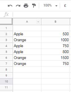
Problem: Sum the Max 2 Sales Quantities of the Fruit “Apple”.
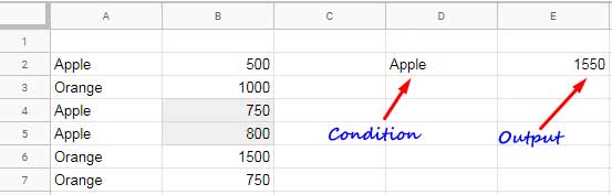
Go through the step-by-step instructions below to know how the formula develops. In the example, the criterion/condition is in cell D2 and the formula in cell E2.
Step # 1: The use of Order by Clause.
The formula in cell E2 that sorts the column B in descending order.
=query(A2:B,"Select * order by B desc")This formula will place the highest values on the top.
Step # 2: The use of Where Clause.
Modify this formula as below.
=query(A2:B,"Select B where A='Apple' order by B desc")Or
=query(A2:B,"Select B where A='"&D2&"' order by B desc")So you have one column with the largest values of the fruit “Apple”
Step # 3: The use of Limit Clause.
We want to sum the largest two values. Modify the formula include the Limit clause and wrap the entire formula with the function SUM.
=sum(query(A2:B,"Select B where A='Apple' order by B desc limit 2"))The above is the final formula to sum large/Max n values based on criteria in Google Sheets. Limit 2 determines the ‘n’ here.
I have used the word “criteria” but used “criterion” in the formula. So if you want to include two conditions, modify the Query as below.
Problem: Sum the Max Two Sales Quantities of the Fruits “Apple” or “Orange”.
=sum(query(A2:B,"Select B where A='Apple' or A='Orange' order by B desc limit 2"))Here the formula finds the max 2 sales quantities from the items “Apple” and “Orange”.
The formula ignores other values (fruits) in column A and then finds the large two values irrespective of the fruits “Apple” or “Orange”
Note:
If you are looking for a formula to sum large two values of each item, I mean large two values of “Apple” and large two values of “Orange”, then you may check my tutorial titled Sum Max n Values Group Wise. The link is given at the end of this tutorial.
SORTN + Filter to Sum Large/Max n Values Based on Conditions
There is another way to sum large/max n values based on conditions in Google Docs Sheets. Here is that.
Here also the criterion “Apple” is in D2 and the formula that I am going to use is in cell E2.
In the first step Filter the dataset for the fruit “Apple”.
=filter(A2:B,A2:A="Apple")Edit this formula to only return the value column.
=filter(B2:B,A2:A="Apple")In the next step, we can SORT the data in descending order and limit the output to ‘n’. Here ‘n’ is two.
=sortn(filter(B2:B,A2:A="Apple"),2,0,1,false)Another formula that uses the Array_Constrain and SORT, that is equivalent to the above.
=array_constrain(sort(filter(B2:B,A2:A="Apple"),1,false),2,1)Wrap the formula with SUM.
=sum(sortn(filter(B2:B,A2:A="Apple"),2,0,1,false))Or
=sum(array_constrain(sort(filter(B2:B,A2:A="Apple"),1,false),2,1))I have the above formula, well explained (I hope so) in my video tutorial below.
Can I use multiple criteria here?
Yes! In both the above formulas, SORTN + Filter or Array_Constrain + SORT + Filter we can bring multiple criteria. Just modify the filter formula for that.
=sum(sortn(filter(B2:B,(A2:A="Apple")+(A2:A="Orange")),2,0,1,false))Here again, take the note given in bold letters above.
Must Read: How to Use AND, OR with Google Sheets Filter Function.
Conclusion
The aim of this tutorial is to make you familiar with how to sum max n values based on criteria in Google Sheets. For that, I have provided two formulas and detailed it as much as I can. Any doubt, please feel free to post in the comments.
Additional Resources:
SHOULD BE NICE IF YOU SHARE A GOOGLE SHEET WITH THIS EXERCISE.
THANKS.