


How to get dynamic column ID in Query Importrange. It may be one of the problems that you may face when using them combined in Google Sheets. Actually, it’s possible with the help of Named Ranges.
When you Query Importrange, use Named Ranges as column identifier or you can say column header in Query. I will explain how to do that. The benefit, if you move a column in the source, it will reflect in the Queried Imported data.
You can Query an Importrange in Google Sheets using Named Ranges.
One of the purposes of using the Query with Importrange is to filter a particular column (Where clause) or select columns (Select clause) or both.
This I have detailed in an earlier Google Spreadsheet tutorial here – How to Use Query With Importrange in Google Sheets.
In such cases, you can see one issue surfacing when you modify your source data. If your selected column or filtered column is shifted in the source, it won’t reflect in the Query Importrange output. Here comes the importance of Named Ranges in Query Importrange.
Similar: Importrange Named Ranges in Google Sheets.
For example, I want to filter column 7 for the value “Completed”. But the formula fails when I insert a new column before column 7. Column 7 moves to 8 (changes position) so the Query Importrange miserably fails to identify that.
How to Get Dynamic Column Id in Query Importrange with Naming Ranges
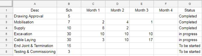
I want to export the below data into a new sheet but only the rows where the Status (column 7) shows “Completed”. How to do that?
Screenshot # 1
This’s not so complicated if you know how to use Query and Importrange together. Here is that formula.
Formula # 1: Query + Importrange.
Note: Replace the URL in all the below formulas with your source file URL.
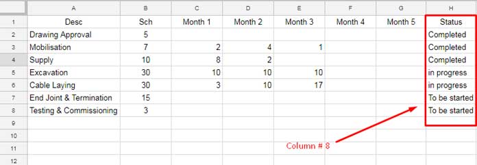
=Query({importrange("URL","Sheet1!A1:G")},"Select * Where Col7 ='Completed'",1)This formula has a problem! In the source insert one column after column 4. This shifts the “Status” column to the right. In the Query Where clause, it won’t reflect.
I mean the changes won’t reflect in the Google Sheets file where you have imported the data conditionally.
Screenshot # 2
As I have told you, you can make the column identifier dynamic in Query Importrange with Named Ranges. Here are the steps.
As a side note, I have a tutorial already regarding the use of Named Ranges in Query – How to Use Named Ranges in Query in Google Sheets. But it doesn’t address the Importrange part. Also, the column identifier is not a column number there but a column letter. I mean not Col7 but G.
Query + Importrange + Named Ranges for Dynamic Column Header/ID
Dynamic Column Id in Query Importrange. Let’s see how to make this a reality.
Steps:
Go to the source and anywhere in that sheet, in a blank cell (you can call it a helper cell) enter the below formula. I am applying this in cell M1. The Column formula returns column number 7.
=column(G1)Column G is the “Status” column. Please refer to
Now name the cell M1 “Status”. You can do that by right-clicking on the cell M1 and selecting “Define named range”
Then we want to define one more range. Select the entire data A1:G8 and name this range as “Source”
Now replace Col7 in the above Query Importrange formula (formula # 1) with the below Importrange Named Ranges formula.
Formula # 2: Importrange Named Range.
=importrange("URL","Status")Then replace the range “Sheet1!A1
The final formula which is a combination of Query + Importrange + Named Ranges will be as follows.
Final Formula: Dynamic Column ID in Query Importrange.
=Query({importrange("URL","Source")},"Select * Where Col"&importrange("URL","Status")&"='Completed'",1)This way you can get dynamic column Id in Query Importrange in Google Sheets.
To test this formula go to the source sheet and insert a column before column G. You can see that the formula correctly point to the moved column.