")
")


")


")

")
")
 in Excel & Google Sheets")


Sometimes, you may want to look up the previous values relative to the current row. For example, in a vehicle list, you can identify the last filled gasoline quantity and compare it with the current quantity to understand how much gasoline was filled during the previous entry. The same formula works seamlessly in both Excel and Google Sheets.
We will use a custom LAMBDA function that incorporates XLOOKUP within the MAP helper function for this task.
Formula to Lookup Previous Values Dynamically in Excel and Google Sheets
Here’s the formula:
=MAP(A1:A10, B1:B10, LAMBDA(Λ,Σ, XLOOKUP(OFFSET(Λ, 1,), A1:Λ, B1:Σ,"",,-1)))A1:A10is the lookup range (e.g., vehicle registration numbers).B1:B10is the result range (e.g., gasoline quantities).A1andB1are the starting rows of your table.
This formula dynamically looks up the current row value within the range up to the previous row and returns the last matching value.
Example: Lookup Previous Values Dynamically
Sample Data:
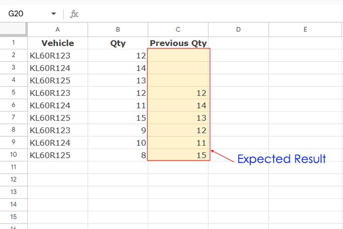
The table contains:
- Vehicle Registration Numbers in column A.
- Gasoline Quantity (gallons) in column B.
The range is A1:B, where A1 and B1 are headers.
To retrieve the last gasoline quantity for each vehicle, enter the following formula in cell C2:
=MAP(A1:A10, B1:B10, LAMBDA(Λ,Σ, XLOOKUP(OFFSET(Λ, 1,), A1:Λ, B1:Σ,"",,-1)))This formula looks up previous values seamlessly in both Excel and Google Sheets.
Formula Breakdown
Before diving deeper, here’s an alternative drag-down formula that achieves the same result:
Enter this XLOOKUP and OFFSET combination formula in cell C2 and drag it down:
=XLOOKUP(OFFSET(A1, 1,), $A$1:A1, $B$1:B1,"",,-1)Explanation:
OFFSET(A1, 1, ):- This is the lookup value (or search key).
- In cell C2, it fetches the value from A2 as the search key.
$A$1:A1:- This is the lookup range, which expands as you drag the formula down.
$B$1:B1:- This is the result range from which the formula retrieves the corresponding value.
- Search Mode
-1:- Ensures the formula searches bottom-to-top in the range for the most recent match.
How It Works:
- In C2, the formula looks up the current row value in A1:A1 and returns the corresponding value from B1:B1.
- When dragged to C3, the formula expands to A1:A2 and B1:B2, effectively searching the prior entries for the most recent match.
This logic is the foundation for looking up previous values in both Excel and Google Sheets.
Automating with a Custom LAMBDA Function
To avoid manual drag-down formulas, we can automate the process using a LAMBDA function:
LAMBDA(Λ,Σ, XLOOKUP(OFFSET(Λ, 1,), A1:Λ, B1:Σ,"",,-1))Explanation of the LAMBDA Function:
Λ: Represents the current element in the first array (A1:A10).Σ: Represents the current element in the second array (B1:B10).
Using the MAP function, this LAMBDA is iterated over both arrays to dynamically compute the previous values for all rows.
Syntax: MAP(array1, [array2, …], lambda)
Key Points:
- MAP Function: Iterates the LAMBDA function over two arrays.
- Greek Letters (
ΛandΣ): Used to avoid conflicts with cell references. - Dynamic Range Expansion: Automatically adjusts lookup ranges for each row.
By combining XLOOKUP with MAP and LAMBDA, you can dynamically lookup previous values in both Excel and Google Sheets without manual intervention.
Additional Resources
- Lookup Last Partial Occurrence in Google Sheets
- Find the Last Occurrence of Multiple Criteria in Google Sheets
- VLOOKUP Last Record in Each Group in Google Sheets
- How to Lookup First and Last Values in a Row in Google Sheets
- Last Row Lookup and Array Results in Google Sheets
- Excel: XLOOKUP for First and Last Non-Blank Value in Row
- Lookup Latest Dates in Google Sheets