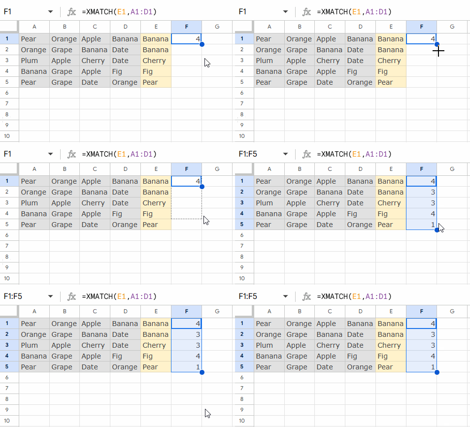
XMATCH Row by Row: Finding Values Across a Range in Google Sheets

Using the BYROW function with XMATCH in Google Sheets allows us to match values row by row across a range, eliminating the need to drag formulas manually. This technique is useful when searching for multiple values in each row and returning the position of each search key within that row’s range.

Example Dataset

Consider the following table in the range A1:D5:

	A	B	C	D
1	Pear	Orange	Apple	Banana
2	Orange	Grape	Banana	Date
3	Plum	Apple	Cherry	Date
4	Banana	Grape	Apple	Fig
5	Pear	Grape	Date	Orange

The search keys we want to locate row by row are in E1:E5:

Banana

Cherry

Fig

Pear

Traditional XMATCH Formula (Row-by-Row Dragging)

Typically, we might use an XMATCH formula like this in F1 and drag it down:

=XMATCH(E1, A1:D1)

XMATCH Drag-Down Formula in Google Sheets

This approach, however, requires manually dragging the formula for each search key, which is inefficient for large datasets. Let’s see how we can use BYROW to apply XMATCH across each row dynamically without dragging.

Step 1: Combining Search Keys and Lookup Range

Since BYROW processes each row independently, we need to structure the data so that each search key aligns with its respective lookup range. This setup ensures that each row’s search key is correctly positioned for XMATCH to locate it within the corresponding range.

In short, BYROW takes a single array_or_range, not multiple ranges. Therefore, we need to combine the search key with the lookup range.

To accomplish this, we can use the HSTACK function to horizontally combine the search keys with the lookup range:

=HSTACK(E1:E5, A1:D5)

This formula stacks the search keys in E1:E5 next to the range A1:D5, creating a new array where each row contains the search key alongside its respective data.

You don’t need to enter this formula directly in the sheet; instead, we’ll use it within the BYROW function in the next step.

Step 2: Applying XMATCH Row by Row with BYROW

The syntax of the BYROW function is as follows:

BYROW(array_or_range, LAMBDA)

Here, array_or_range will be the result of our HSTACK formula from Step 1. In the LAMBDA function, we’ll use XMATCH to perform a row-by-row lookup.

XMATCH for Finding Values Across a Range:

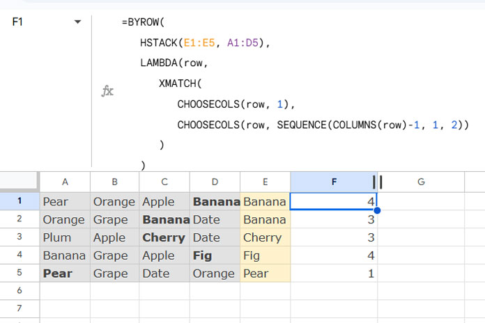
=BYROW(
   HSTACK(E1:E5, A1:D5), 
   LAMBDA(row, 
      XMATCH(
         CHOOSECOLS(row, 1), 
         CHOOSECOLS(row, SEQUENCE(COLUMNS(row)-1, 1, 2))
      )
   )
)

This formula finds the position of each search key within its respective row without requiring any manual dragging. Let’s break down each part of this formula to understand its function.

XMATCH Row by Row in Google Sheets Using BYROW Function

Explanation of the Custom LAMBDA Function with XMATCH

Here is the custom LAMBDA function in use:

LAMBDA(row, 
      XMATCH(
         CHOOSECOLS(row, 1), 
         CHOOSECOLS(row, SEQUENCE(COLUMNS(row)-1, 1, 2))
      )
   )

Where:

LAMBDA(row, …): Defines row as the variable representing each row processed by BYROW.
XMATCH(CHOOSECOLS(row, 1), CHOOSECOLS(row, SEQUENCE(COLUMNS(row)-1, 1, 2))):
- CHOOSECOLS(row, 1): Extracts the first column (the search key) from each row.
- CHOOSECOLS(row, SEQUENCE(COLUMNS(row)-1, 1, 2)): Selects all columns after the first column, creating the lookup range for XMATCH within each row.

The XMATCH function searches for the search key in the remaining columns (lookup range) of each row, providing a dynamic, row-by-row solution.

Formula Summary

XMATCH Syntax: XMATCH(search_key, lookup_range, [match_mode], [search_mode])
- search_key: CHOOSECOLS(row, 1) — the first column, which is the search key.
- lookup_range: CHOOSECOLS(row, SEQUENCE(COLUMNS(row)-1, 1, 2)) — the remaining columns within each row.

This approach enables XMATCH to search each row individually within the specified range, making the lookup process both dynamic and efficient.

This method is especially helpful in applications like inventory checks, attendance tracking, or any scenario where row-wise lookups are needed across multiple columns in Google Sheets.